
On The Performance of Hashing for Similar Function Detection
Imagine that you reverse engineered a piece of malware in pain-staking detail, only to find that the malware author created a slightly modified version of the malware the next day. You wouldn't want to redo all your hard work. One way to avoid this is to use code comparison techniques to try to identify pairs of functions in the old and new version that are "the same" (which I put in quotes because it's a bit of a nebulous concept, as we'll see).
There are several tools to help in such situations. A very popular (formerly) commercial tool is zynamics' bindiff, which is now owned by Google and free. CMU SEI's Pharos also includes a code comparison utility called fn2hash, which is the subject of this blog post.
Background
Exact Hashing
fn2hash employs several types of hashing, with the most commonly used one called PIC hashing, where PIC stands for Position Independent Code. To see why PIC hashing is important, we'll actually start by looking at a naive precursor to PIC hashing, which is to simply hash the instruction bytes of a function. We'll call this exact hashing.
Let's look at an example. I compiled this simple program
oo.cpp with
g++. Here's the beginning of the assembly code for the function myfunc
(full
code):
Assembly code and bytes from oo.gcc
;;;;;;;;;;;;;;;;;;;;;;;;;;;;;;;;;;;;;;;;;;;;;;;;;;;;;;;;;;;;;;;;;;;;;;;;;;;;;;;;;;;;;;;;;;;;;;;;;;;;;;;;;;;;;;;;;;;;;;;;
;;; function 0x00401200 "myfunc()"
;;; mangled name is "_Z6myfuncv"
;;; reasons for function: referenced by symbol table

;; predecessor:  from instruction 0x004010f4 from basic block 0x004010f0
0x00401200: 41 56                      00 push     r140x00401202: bf 60 00 00 00            -08 mov      edi, 0x00000060<96>
0x00401207: 41 55                     -08 push     r13
0x00401209: 41 54                     -10 push     r12
0x0040120b: 55                        -18 push     rbp
0x0040120c: 48 83 ec 08               -20 sub      rsp, 8
0x00401210: e8 bb fe ff ff            -28 call     function 0x004010d0 "operator new(unsigned long)@plt"
Exact Bytes
In the first highlighted line, you can see that the first instruction is a
push r14, which is encoded by the instruction bytes 41 56. If we collect the
encoded instruction bytes for every instruction in the function, we get:
Exact bytes in oo.gcc
4156BF6000000041554154554883EC08E8BBFEFFFFBF6000000048C700F02040004889C548C7401010214000C740582A000000E898FEFFFFBF1000000048C700F02040004989C448C7401010214000C740582A000000E875FEFFFFBA0D000000BE48204000BF80404000C74008000000004989C5C6400C0048C700D8204000E82CFEFFFF488B05F52D0000488B40E84C8BB0704140004D85F60F842803000041807E38000F84160200004C89F7E898FBFFFF498B06BE0A000000488B4030483DD01540000F84CFFDFFFF4C89F7FFD00FBEF0E9C2FDFFFF410FBE7643BF80404000E827FEFFFF4889C7E8FFFDFFFF488B4500488B00483DE01740000F85AC0200004889EFFFD0488B4500488B4008483D601640000F84A0FDFFFFBA0D000000BE3A204000BF80404000E8C8FDFFFF488B05912D0000488B40E84C8BB0704140004D85F60F84C402000041807E38000F84820100004C89F7E8C8FBFFFF498B06BE0A000000488B4030483DD01540000F8463FEFFFF4C89F7FFD00FBEF0E956FEFFFF410FBE7643BF80404000E8C3FDFFFF4889C7E89BFDFFFF488B4500488B4008483D601640000F85600200004889EFFFD0E9E7FDFFFFBA0D000000BE1E204000BF80404000E863FDFFFF488B052C2D0000488B40E84C8BB0704140004D85F60F845F02000041807E38000F847D0100004C89F7E868FBFFFF498B06BE0A000000488B4030483DD01540000F8468FEFFFF4C89F7FFD00FBEF0E95BFEFFFF410FBE7643BF80404000E85EFDFFFF4889C7E836FDFFFF488B4510488D7D10488B4008483DE01540000F8506020000FFD0498B0424488B00483DE01740000F8449FEFFFFBA0D000000BE10204000BF80404000E8FAFCFFFF488B05C32C0000488B40E84C8BB0704140004D85F60F84F601000041807E38000F84440100004C89F7E838FBFFFF498B06BE0A000000488B4030483DD01540000F84A1FEFFFF4C89F7FFD00FBEF0E994FEFFFF410FBE7643BF80404000E8F5FCFFFF4889C7E8CDFCFFFF498B0424488B00483DE01740000F85B70100004C89E7FFD0E990FEFFFFBA0D000000BE3A204000BF80404000E896FCFFFF488B055F2C0000488B40E84C8BB0704140004D85F60F8492010000E864FAFFFF0F1F400041807E38000F84100100004C89F7E808FBFFFF498B06BE0A000000488B4030483DD01540000F84D5FEFFFF4C89F7FFD00FBEF0E9C8FEFFFF410FBE7643BF80404000E891FCFFFF4889C7E869FCFFFF4889EFBE60000000E8FC0300004C89E7BE10000000E8EF0300004883C4084C89EFBE100000005D415C415D415EE9D7030000We call this sequence the exact bytes of the function. We can hash these bytes to get an exact hash, 62CE2E852A685A8971AF291244A1283A.
Short-comings of Exact Hashing
The highlighted call at address 0x401210 is a relative call, which means that
the target is specified as an offset from the current instruction (well,
technically the next instruction). If you look at the instruction bytes for this
instruction, it includes the bytes bb fe ff ff, which is 0xfffffebb in little
endian form; interpreted as a signed integer value, this is -325. If we take
the address of the next instruction (0x401210 + 5 == 0x401215) and then add -325
to it, we get 0x4010d0, which is the address of operator new, the target of
the call. Yay. So now we know that bb fe ff ff is an offset from the next
instruction. Such offsets are called relative offsets because they are
relative to the address of the next instruction.
I created a slightly modified
program (oo2.gcc) by
adding an empty, unused function before myfunc. You can find the disassembly
of myfunc for this executable
here.
If we take the exact hash of myfunc in this new executable, we get
05718F65D9AA5176682C6C2D5404CA8D. Wait, that's different than the hash for
myfunc in the first executable, 62CE2E852A685A8971AF291244A1283A. What
happened? Let's look at the disassembly.
Assembly code and bytes from oo2.gcc
;;;;;;;;;;;;;;;;;;;;;;;;;;;;;;;;;;;;;;;;;;;;;;;;;;;;;;;;;;;;;;;;;;;;;;;;;;;;;;;;;;;;;;;;;;;;;;;;;;;;;;;;;;;;;;;;;;;;;;;;
;;; function 0x00401210 "myfunc()"

;; predecessor:  from instruction 0x004010f4 from basic block 0x004010f0
0x00401210: 41 56                      00 push     r14
0x00401212: bf 60 00 00 00            -08 mov      edi, 0x00000060<96>
0x00401217: 41 55                     -08 push     r13
0x00401219: 41 54                     -10 push     r12
0x0040121b: 55                        -18 push     rbp
0x0040121c: 48 83 ec 08               -20 sub      rsp, 8
0x00401220: e8 ab fe ff ff            -28 call     function 0x004010d0 "operator new(unsigned long)@plt"
Notice that myfunc moved from 0x401200 to 0x401210, which also moved the
address of the call instruction from 0x401210 to 0x401220. Because the call
target is specified as an offset from the (next) instruction's address, which
changed by 0x10 == 16, the offset bytes for the call changed from bb fe ff ff
(-325) to ab fe ff ff (-341 == -325 - 16). These changes modify the exact
bytes to:
Exact bytes in oo2.gcc
4156BF6000000041554154554883EC08E8ABFEFFFFBF6000000048C700F02040004889C548C7401010214000C740582A000000E888FEFFFFBF1000000048C700F02040004989C448C7401010214000C740582A000000E865FEFFFFBA0D000000BE48204000BF80404000C74008000000004989C5C6400C0048C700D8204000E81CFEFFFF488B05E52D0000488B40E84C8BB0704140004D85F60F842803000041807E38000F84160200004C89F7E888FBFFFF498B06BE0A000000488B4030483DE01540000F84CFFDFFFF4C89F7FFD00FBEF0E9C2FDFFFF410FBE7643BF80404000E817FEFFFF4889C7E8EFFDFFFF488B4500488B00483DF01740000F85AC0200004889EFFFD0488B4500488B4008483D701640000F84A0FDFFFFBA0D000000BE3A204000BF80404000E8B8FDFFFF488B05812D0000488B40E84C8BB0704140004D85F60F84C402000041807E38000F84820100004C89F7E8B8FBFFFF498B06BE0A000000488B4030483DE01540000F8463FEFFFF4C89F7FFD00FBEF0E956FEFFFF410FBE7643BF80404000E8B3FDFFFF4889C7E88BFDFFFF488B4500488B4008483D701640000F85600200004889EFFFD0E9E7FDFFFFBA0D000000BE1E204000BF80404000E853FDFFFF488B051C2D0000488B40E84C8BB0704140004D85F60F845F02000041807E38000F847D0100004C89F7E858FBFFFF498B06BE0A000000488B4030483DE01540000F8468FEFFFF4C89F7FFD00FBEF0E95BFEFFFF410FBE7643BF80404000E84EFDFFFF4889C7E826FDFFFF488B4510488D7D10488B4008483DF01540000F8506020000FFD0498B0424488B00483DF01740000F8449FEFFFFBA0D000000BE10204000BF80404000E8EAFCFFFF488B05B32C0000488B40E84C8BB0704140004D85F60F84F601000041807E38000F84440100004C89F7E828FBFFFF498B06BE0A000000488B4030483DE01540000F84A1FEFFFF4C89F7FFD00FBEF0E994FEFFFF410FBE7643BF80404000E8E5FCFFFF4889C7E8BDFCFFFF498B0424488B00483DF01740000F85B70100004C89E7FFD0E990FEFFFFBA0D000000BE3A204000BF80404000E886FCFFFF488B054F2C0000488B40E84C8BB0704140004D85F60F8492010000E854FAFFFF0F1F400041807E38000F84100100004C89F7E8F8FAFFFF498B06BE0A000000488B4030483DE01540000F84D5FEFFFF4C89F7FFD00FBEF0E9C8FEFFFF410FBE7643BF80404000E881FCFFFF4889C7E859FCFFFF4889EFBE60000000E8FC0300004C89E7BE10000000E8EF0300004883C4084C89EFBE100000005D415C415D415EE9D7030000You can look through that and see the differences by eyeballing it. Just kidding! Here's a visual comparison. Red represents bytes that are only in oo.gcc, and green represents bytes in oo2.gcc. The differences are small because the offset is only changing by 0x10, but this is enough to break exact hashing.
Difference between exact bytes in oo.gcc and oo2.gcc
4156BF6000000041554154554883EC08E8BBABFEFFFFBF6000000048C700F02040004889C548C7401010214000C740582A000000E89888FEFFFFBF1000000048C700F02040004989C448C7401010214000C740582A000000E87565FEFFFFBA0D000000BE48204000BF80404000C74008000000004989C5C6400C0048C700D8204000E82C1CFEFFFF488B05F5E52D0000488B40E84C8BB0704140004D85F60F842803000041807E38000F84160200004C89F7E89888FBFFFF498B06BE0A000000488B4030483DD0E01540000F84CFFDFFFF4C89F7FFD00FBEF0E9C2FDFFFF410FBE7643BF80404000E82717FEFFFF4889C7E8FFEFFDFFFF488B4500488B00483DE0F01740000F85AC0200004889EFFFD0488B4500488B4008483D60701640000F84A0FDFFFFBA0D000000BE3A204000BF80404000E8C8B8FDFFFF488B0591812D0000488B40E84C8BB0704140004D85F60F84C402000041807E38000F84820100004C89F7E8C8B8FBFFFF498B06BE0A000000488B4030483DD0E01540000F8463FEFFFF4C89F7FFD00FBEF0E956FEFFFF410FBE7643BF80404000E8C3B3FDFFFF4889C7E89B8BFDFFFF488B4500488B4008483D60701640000F85600200004889EFFFD0E9E7FDFFFFBA0D000000BE1E204000BF80404000E86353FDFFFF488B052C1C2D0000488B40E84C8BB0704140004D85F60F845F02000041807E38000F847D0100004C89F7E86858FBFFFF498B06BE0A000000488B4030483DD0E01540000F8468FEFFFF4C89F7FFD00FBEF0E95BFEFFFF410FBE7643BF80404000E85E4EFDFFFF4889C7E83626FDFFFF488B4510488D7D10488B4008483DE0F01540000F8506020000FFD0498B0424488B00483DE0F01740000F8449FEFFFFBA0D000000BE10204000BF80404000E8FAEAFCFFFF488B05C3B32C0000488B40E84C8BB0704140004D85F60F84F601000041807E38000F84440100004C89F7E83828FBFFFF498B06BE0A000000488B4030483DD0E01540000F84A1FEFFFF4C89F7FFD00FBEF0E994FEFFFF410FBE7643BF80404000E8F5E5FCFFFF4889C7E8CDBDFCFFFF498B0424488B00483DE0F01740000F85B70100004C89E7FFD0E990FEFFFFBA0D000000BE3A204000BF80404000E89686FCFFFF488B055F4F2C0000488B40E84C8BB0704140004D85F60F8492010000E86454FAFFFF0F1F400041807E38000F84100100004C89F7E808FBF8FAFFFF498B06BE0A000000488B4030483DD0E01540000F84D5FEFFFF4C89F7FFD00FBEF0E9C8FEFFFF410FBE7643BF80404000E89181FCFFFF4889C7E86959FCFFFF4889EFBE60000000E8FC0300004C89E7BE10000000E8EF0300004883C4084C89EFBE100000005D415C415D415EE9D7030000
PIC Hashing
This problem is the motivation for few different types of hashing that we'll
talk about in this blog post, including PIC hashing and fuzzy hashing. The
PIC in PIC hashing stands for Position Independent Code. At a high level,
the goal of PIC hashing is to compute a hash or signature of code, but do so in
a way that relocating the code will not change the hash. This is important
because, as we just saw, modifying a program often results in small changes to
addresses and offsets and we don't want these changes to modify the hash!. The
intuition behind PIC hashing is very straight-forward: identify offsets and
addresses that are likely to change if the program is recompiled, such as bb fe ff ff,
and simply set them to zero before hashing the bytes. That way if they
change because the function is relocated, the function's PIC hash won't change.
The following visual diff shows the differences between the exact bytes and the
PIC bytes on myfunc in oo.gcc. Red represents bytes that are only in the PIC
bytes, and green represents the exact bytes. As expected, the first
change we can see is the byte sequence bb fe ff ff, which is changed to zeros.
Byte difference between PIC bytes (red) and exact bytes (green)
4156BF6000000041554154554883EC08E800000000BBFEFFFFBF6000000048C700000000F02040004889C548C7401000000010214000C740582A000000E80000000098FEFFFFBF1000000048C700000000F02040004989C448C7401000000010214000C740582A000000E80000000075FEFFFFBA0D000000BE00000048204000BF00000080404000C74008000000004989C5C6400C0048C700000000D8204000E8000000002CFEFFFF488B050000F52D0000488B40E84C8BB0000000704140004D85F60F842803000041807E38000F84160200004C89F7E80000000098FBFFFF498B06BE0A000000488B4030483D000000D01540000F84CFFDFFFF4C89F7FFD00FBEF0E9C2FDFFFF410FBE7643BF00000080404000E80000000027FEFFFF4889C7E800000000FFFDFFFF488B4500488B00483D000000E01740000F85AC0200004889EFFFD0488B4500488B4008483D000000601640000F84A0FDFFFFBA0D000000BE0000003A204000BF00000080404000E800000000C8FDFFFF488B050000912D0000488B40E84C8BB0000000704140004D85F60F84C402000041807E38000F84820100004C89F7E800000000C8FBFFFF498B06BE0A000000488B4030483D000000D01540000F8463FEFFFF4C89F7FFD00FBEF0E956FEFFFF410FBE7643BF00000080404000E800000000C3FDFFFF4889C7E8000000009BFDFFFF488B4500488B4008483D000000601640000F85600200004889EFFFD0E9E7FDFFFFBA0D000000BE0000001E204000BF00000080404000E80000000063FDFFFF488B0500002C2D0000488B40E84C8BB0000000704140004D85F60F845F02000041807E38000F847D0100004C89F7E80000000068FBFFFF498B06BE0A000000488B4030483D000000D01540000F8468FEFFFF4C89F7FFD00FBEF0E95BFEFFFF410FBE7643BF00000080404000E8000000005EFDFFFF4889C7E80000000036FDFFFF488B4510488D7D10488B4008483D000000E01540000F8506020000FFD0498B0424488B00483D000000E01740000F8449FEFFFFBA0D000000BE00000010204000BF00000080404000E800000000FAFCFFFF488B050000C32C0000488B40E84C8BB0000000704140004D85F60F84F601000041807E38000F84440100004C89F7E80000000038FBFFFF498B06BE0A000000488B4030483D000000D01540000F84A1FEFFFF4C89F7FFD00FBEF0E994FEFFFF410FBE7643BF00000080404000E800000000F5FCFFFF4889C7E800000000CDFCFFFF498B0424488B00483D000000E01740000F85B70100004C89E7FFD0E990FEFFFFBA0D000000BE0000003A204000BF00000080404000E80000000096FCFFFF488B0500005F2C0000488B40E84C8BB0000000704140004D85F60F8492010000E80000000064FAFFFF0F1F400041807E38000F84100100004C89F7E80000000008FBFFFF498B06BE0A000000488B4030483D000000D01540000F84D5FEFFFF4C89F7FFD00FBEF0E9C8FEFFFF410FBE7643BF00000080404000E80000000091FCFFFF4889C7E80000000069FCFFFF4889EFBE60000000E80000FC0300004C89E7BE10000000E80000EF0300004883C4084C89EFBE100000005D415C415D415EE90000D7030000
If we hash the PIC bytes, we get the PIC hash
EA4256ECB85EDCF3F1515EACFA734E17. And, as we would hope, we get the same PIC
hash for myfunc in the slightly modified oo2.gcc.
Evaluating the Accuracy of PIC Hashing
The primary motivation behind PIC hashing is to detect identical code that is moved to a different location. But what if two pieces of code are compiled with different compilers or different compiler flags? What if two functions are very similar, but one has a line of code removed? Because these changes would modify the non-offset bytes that are used in the PIC hash, it would change the PIC hash of the code. Since we know that PIC hashing will not always work, in this section we'll discuss how we can measure the performance of PIC hashing and compare it to other code comparison techniques.
Before we can define the accuracy of any code comparison technique, we'll need some ground truth that tells us which functions are equivalent. For this blog post, we'll use compiler debug symbols to map function addresses to their names. This will provide us with a ground truth set of functions and their names. For the purposes of this blog post, and general expediency, we'll assume that if two functions have the same name, they are "the same". (This obviously is not true in general!)
Confusion Matrices
So, let's say we have two similar executables, and we want to evaluate how well PIC hashing can identify equivalent functions across both executables. We'll start by considering all possible pairs of functions, where each pair contains a function from each executable. If we're being mathy, this is called the cartesian product (between the functions in the first executable and the functions in the second executable). For each function pair, we'll use the ground truth to determine if the functions are the same by seeing if they have the same name. Then we'll use PIC hashing to predict whether the functions are the same by computing their hashes and seeing if they are identical. There are two outcomes for each determination, so there are four possibilities in total:
- True Positive (TP): PIC hashing correctly predicted the functions are equivalent.
- True Negative (TN): PIC hashing correctly predicted the functions are different.
- False Positive (FP): PIC hashing incorrectly predicted the functions are equivalent, but they are not.
- False Negative (FN): PIC hashing incorrectly predicted the functions are different, but they are equivalent.
To make it a little easier to interpret, we color the good outcomes green and the bad outcomes red.
We can represent these in what is called a confusion matrix:
| Hashing says same | Hashing says different | |
|---|---|---|
| Ground truth says same | TP | FN |
| Ground truth says different | FP | TN |
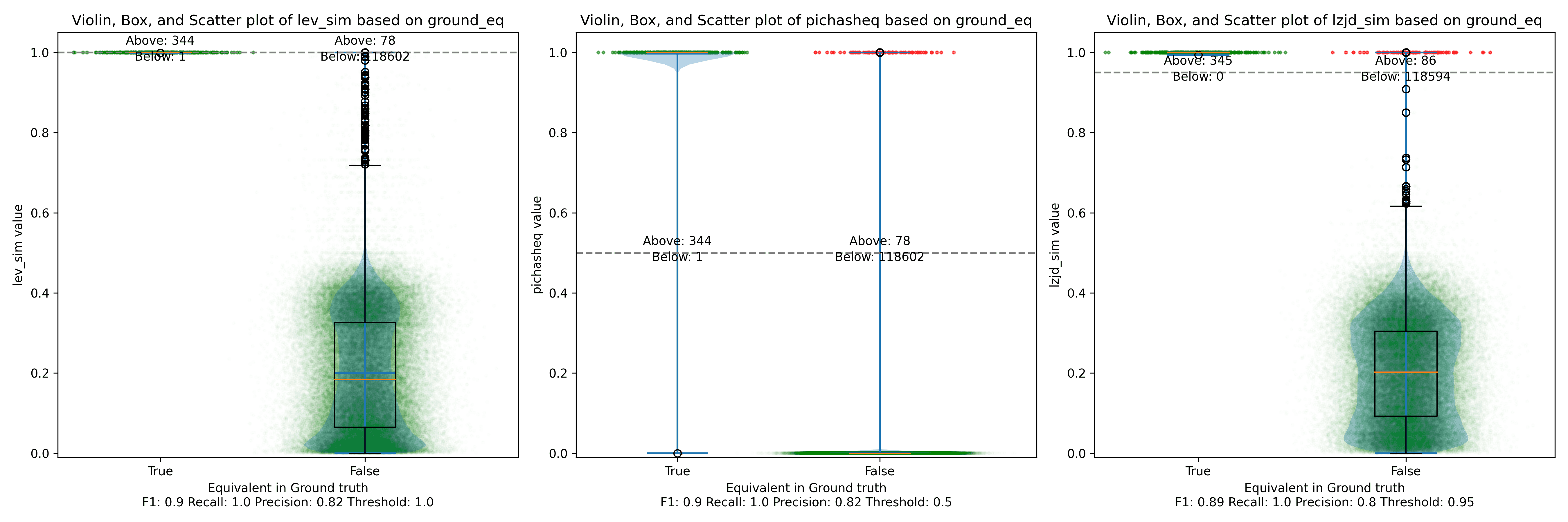
For example, here is a confusion matrix from an experiment where I use PIC hashing to compare openssl versions 1.1.1w and 1.1.1v when they are both compiled in the same manner. These two versions of openssl are very similar, so we would expect that PIC hashing would do well because a lot of functions will be identical but shifted to different addresses. And, indeed, it does:
| Hashing says same | Hashing says different | |
|---|---|---|
| Ground truth says same | 344 | 1 |
| Ground truth says different | 78 | 118,602 |
Metrics: Accuracy, Precision, and Recall
So when does PIC hashing work well, and when does it not? In order to answer these questions, we're going to need an easier way to evaluate the quality of a confusion matrix as a single number. At first glance, accuracy seems like the most natural metric, which tell us: How many pairs did hashing predict correctly? This is equal to
For the above example, PIC hashing achieved an accuracy of
99.9% accuracy. Pretty good, right?
But if you look closely, there's a subtle problem. Most function pairs are not equivalent. According to the ground truth, there are equivalent function pairs, and non-equivalent function pairs. So, if we just guessed that all function pairs were non-equivalent, we would still be right of the time. Since accuracy weights all function pairs equally, it is not the best metric here.
Instead, we want a metric that emphasizes positive results, which in this case are equivalent function pairs. This is consistent with our goal in reverse engineering, because knowing that two functions are equivalent allows a reverse engineer to transfer knowledge from one executable to another and save time!
Three metrics that focus more on positive cases (i.e., equivalent functions) are precision, recall, and F1 score:
- Precision: Of the function pairs hashing declared equivalent, how many were actually equivalent? This is equal to .
- Recall: Of the equivalent function pairs, how many did hashing correctly declare as equivalent? This is equal to .
- F1 score: This is a single metric that reflects both the Precision and Recall. Specifically, it is the harmonic mean of the Precision and Recall, or . Compared to the arithmetic mean, the harmonic mean is more sensitive to low values. This means that if either Precision or Recall is low, the F1 score will also be low.
So, looking at the above example, we can compute the precision, recall, and F1 score. The precision is , the recall is , and the F1 score is . So, PIC hashing is able to identify 81% of equivalent function pairs, and when it does declare a pair is equivalent, it is correct 99.7% of the time. This corresponds to a F1 score of 0.89 out of 1.0, which is pretty good!
Now, you might be wondering how well PIC hashing performs when the differences between executables are larger.
Let's look at another experiment. In this one, I compare an openssl executable compiled with gcc to one compiled with clang. Because gcc and clang generate assembly code differently, we would expect there to be a lot more differences.
Here is a confusion matrix from this experiment:
| Hashing says same | Hashing says different | |
|---|---|---|
| Ground truth says same | 23 | 301 |
| Ground truth says different | 31 | 117,635 |
In this example, PIC hashing achieved a recall of , and a precision of . So, hashing is only able to identify 7% of equivalent function pairs, but when it does declare a pair is equivalent, it is correct 43% of the time. This corresponds to a F1 score of 0.12 out of 1.0, which is pretty bad. Imagine that you spent hours reverse engineering the 324 functions in one of the executables, only to find that PIC hashing was only able to identify 23 of them in the other executable, so you would be forced to needlessly reverse engineer the other functions from scratch. That would be pretty frustrating! Can we do better?
The Great Fuzzy Hashing Debate
There's a very different type of hashing called fuzzy hashing. Like regular
hashing, there is a hash function that reads a sequence of bytes and produces a hash.
Unlike regular hashing, though, you don't compare fuzzy hashes with equality.
Instead, there is a similarity function which takes two fuzzy hashes as input,
and returns a number between 0 and 1, where 0 means completely dissimilar, and 1
means completely similar.
My colleague, Cory Cohen, and I, actually debated whether there is utility in applying fuzzy hashes to instruction bytes, and our debate motivated this blog post. I thought there would be a benefit, but Cory felt there would not. Hence these experiments! For this blog post, I'll be using the Lempel-Ziv Jaccard Distance fuzzy hash, or just LZJD for short, because it's very fast. Most fuzzy hash algorithms are pretty slow. In fact, learning about LZJD is what motivated our debate. The possibility of a fast fuzzy hashing algorithm opens up the possibility of using fuzzy hashes to search for similar functions in a large database and other interesting possibilities.
I'll also be using Levenshtein distance as a baseline. Levenshtein distance is a measure of how many changes you need to make to one string to transform it to another. For example, the Levenshtein distance between "cat" and "bat" is 1, because you only need to change the first letter. Levenshtein distance allows us to define an optimal notion of similarity at the instruction byte level. The trade-off is that it's really slow, so it's only really useful as a baseline in our experiments.
Experiments
To test the accuracy of PIC hashing under various scenarios, I defined a few experiments. Each experiment takes a similar (or identical) piece of source code and compiles it, sometimes with different compilers or flags.
Experiment 1: openssl 1.1.1w
In this experiment, I compiled openssl 1.1.1w in a few different ways. In each
case, I examined the resulting openssl executable.
Experiment 1a: openssl1.1.1w Compiled With Different Compilers
In this first experiment, I compiled openssl 1.1.1w with gcc -O3 -g and clang
-O3 -g and compared the results. We'll start with the confusion matrix for PIC
hashing:
| Hashing says same | Hashing says different | |
|---|---|---|
| Ground truth says same | 23 | 301 |
| Ground truth says different | 31 | 117,635 |
As we saw earlier, this results in a recall of 0.07, a precision of 0.45, and a F1 score of 0.12. To summarize: pretty bad.
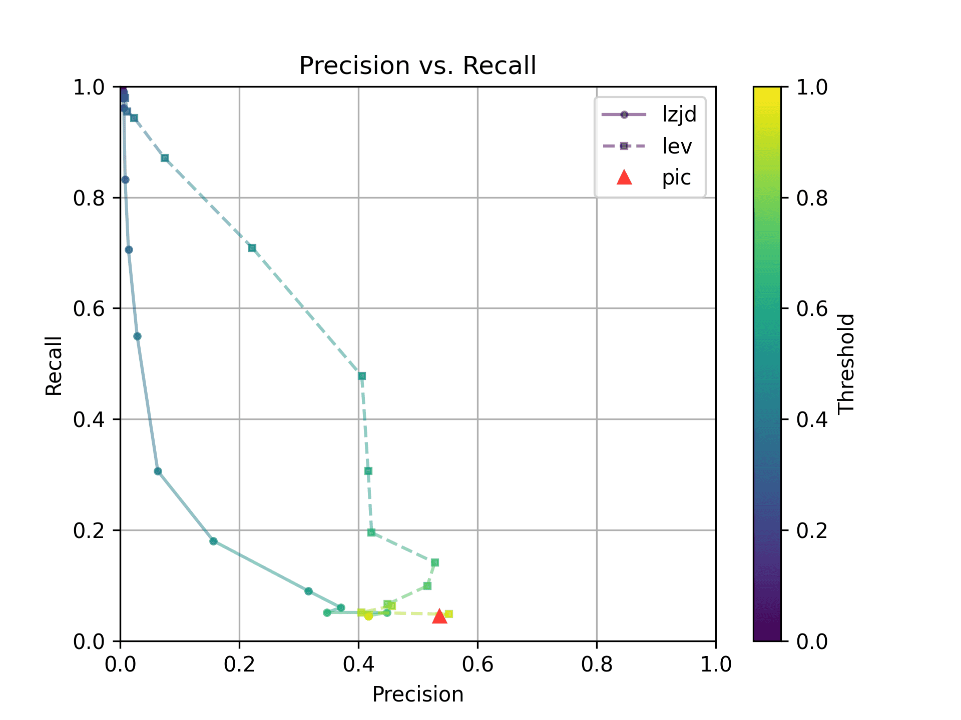
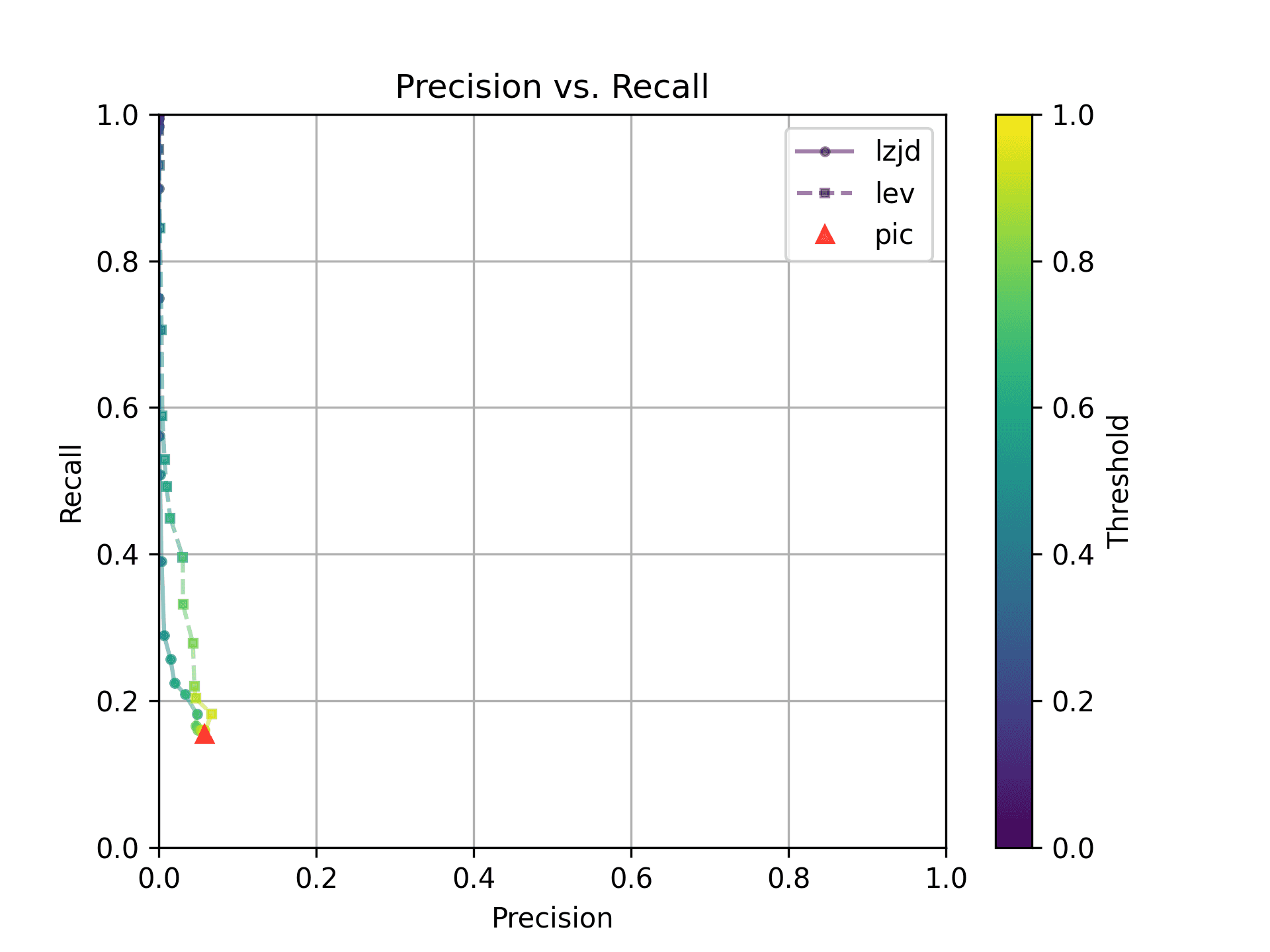
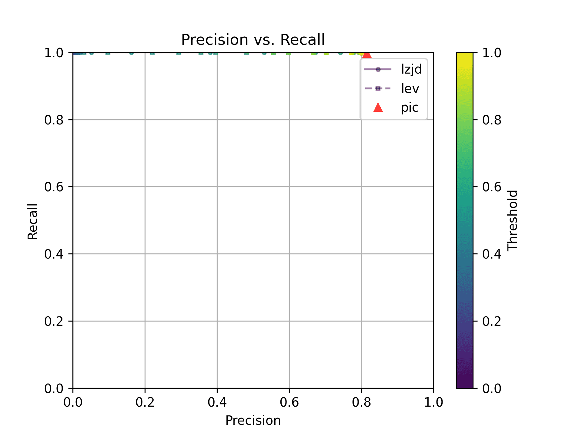
How do LZJD and LEV do? Well, that's a bit harder to quantify, because we have to pick a similarity threshold at which we consider the function to be "the same". For example, at a threshold of 0.8, we'd consider a pair of functions to be the same if they had a similarity score of 0.8 or higher. To communicate this information, we could output a confusion matrix for each possible threshold. Instead of doing this, I'll plot the results for a range of thresholds below:
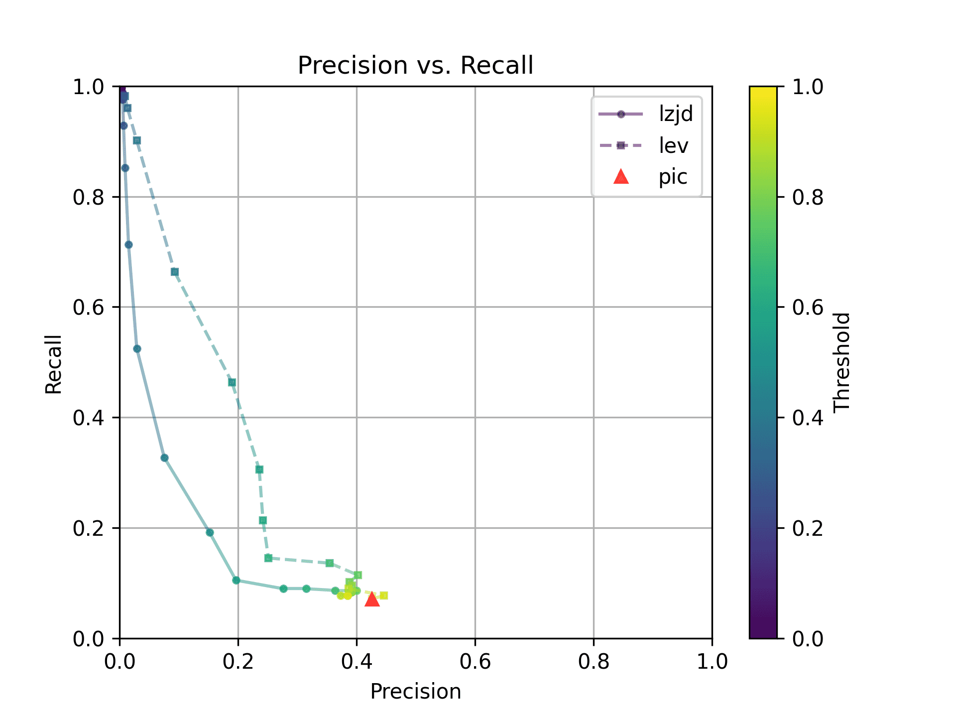
The red triangle represents the precision and recall of PIC hashing: 0.45 and 0.07 respectively, just like we got above. The solid line represents the performance of LZJD, and the dashed line represents the performance of LEV (Levenshtein distance). The color tells us what threshold is being used for LZJD and LEV. On this graph, the ideal result would be at the top right (100% recall and precision). So, for LZJD and LEV to have an advantage, it should be above or to the right of PIC hashing. But we can see that both LZJD and LEV go sharply to the left before moving up, which indicates that a substantial decrease in precision is needed to improve recall.
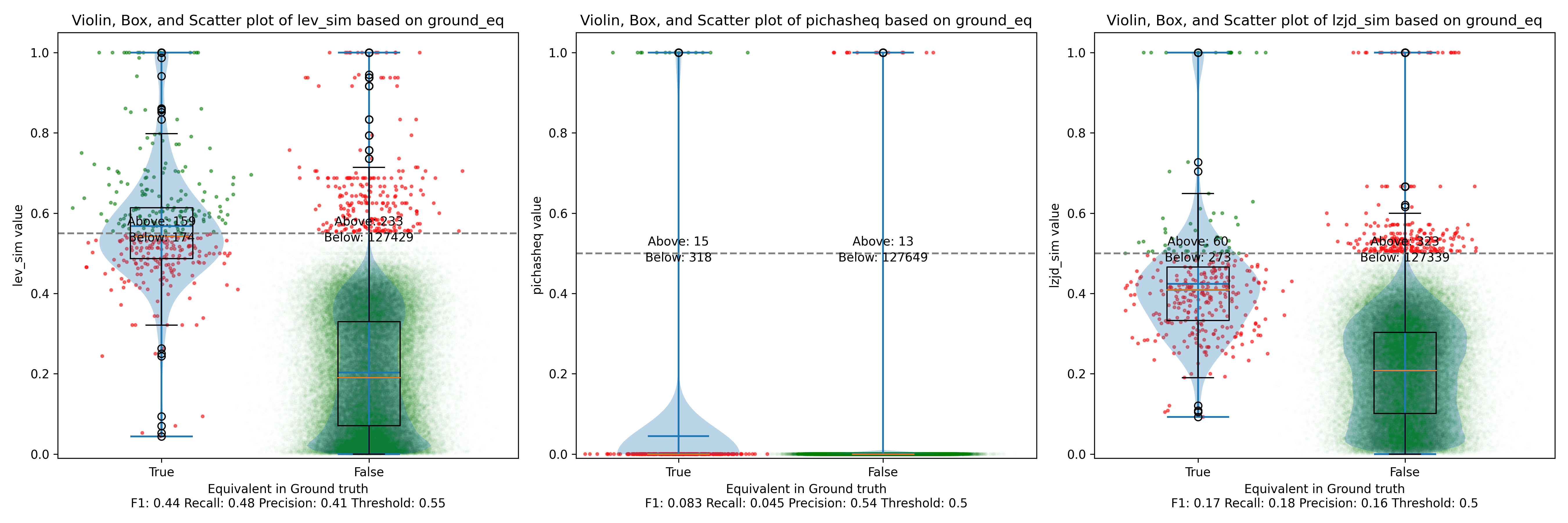
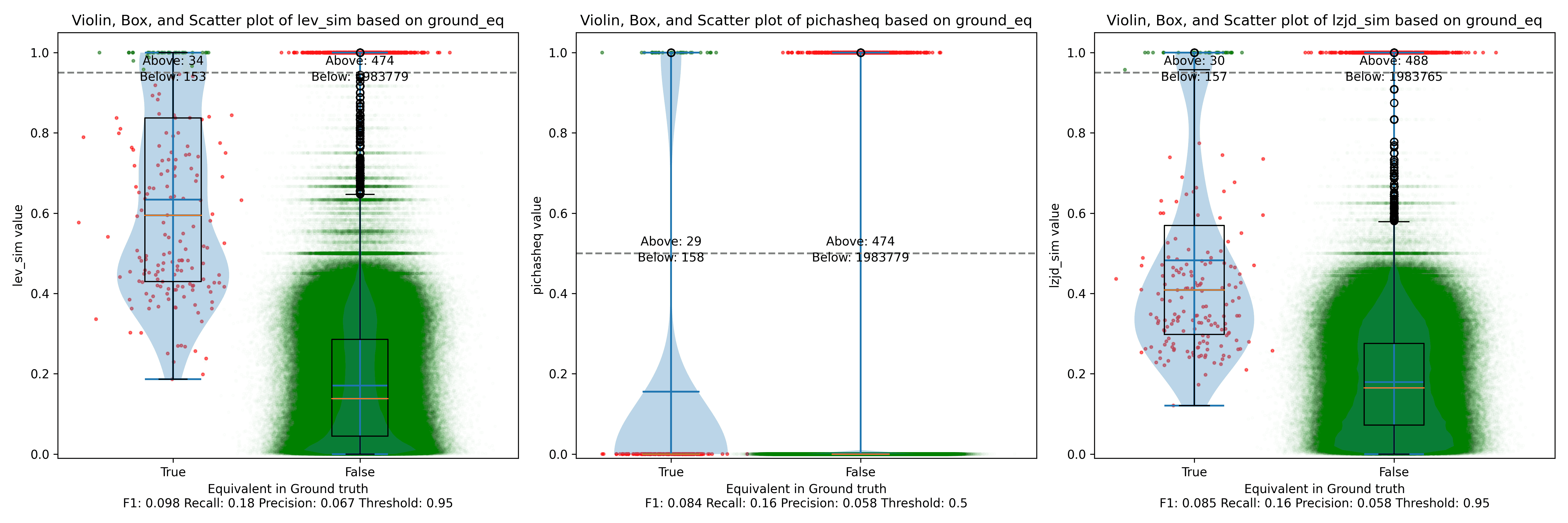
Below is what I call the violin plot. You may want to click on it to zoom in, since it's pretty wide and my blog layout is not. I also spent a long time getting that to work! There are three panels: the leftmost is for LEV, the middle is for PIC hashing, and the rightmost is for LZJD. On each panel, there is a True column, which shows the distribution of similarity scores for equivalent pairs of functions. There is also a False column, which shows the distribution scores for non-equivalent pairs of functions. Since PIC hashing does not provide a similarity score, we consider every pair to be either equivalent (1.0) or not (0.0). A horizontal dashed line is plotted to show the threshold that has the highest F1 score (i.e., a good combination of both precision and recall). Green points indicate function pairs that are correctly predicted as equivalent or not, whereas red points indicate mistakes.
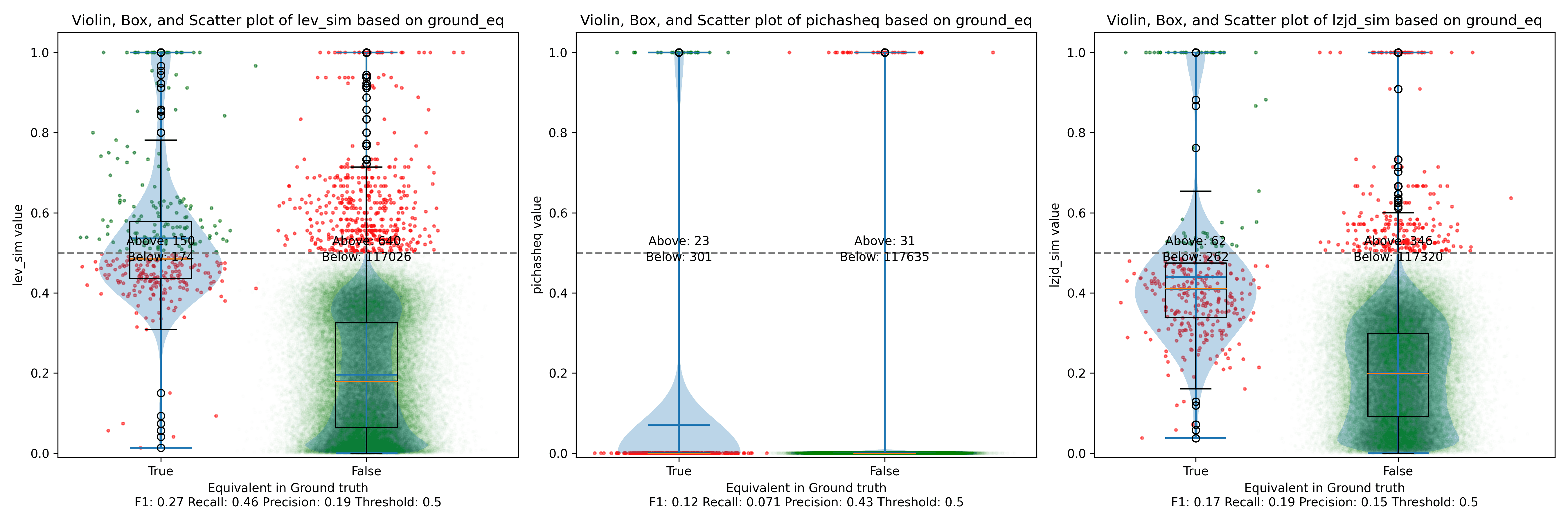
I like this visualization because it shows how well each similarity metric differentiates the similarity distributions of equivalent and non-equivalent function pairs. Obviously, the hallmark of a good similarity metric is that the distribution of equivalent functions should be higher than non-equivalent functions! Ideally, the similarity metric should produce distributions that do not overlap at all, so we could draw a line between them. In practice, the distributions usually intersect, and so instead we're forced to make a trade-off between precision and recall, as can be seen in the above Precision vs. Recall graph.
Overall, we can see from the violin plot that LEV and LZJD have a slightly
higher F1 score (reported at the bottom of the violin plot), but none of these
techniques are doing a great job. This implies that gcc and clang produce
code that is quite different syntactically.
Experiment 1b: openssl 1.1.1w Compiled With Different Optimization Levels
The next comparison I did was to compile openssl 1.1.1w with gcc -g and
optimization levels -O0, -O1, -O2, -O3.
-O0 and -O3
Let's start with one of the extremes, comparing -O0 and -O3:
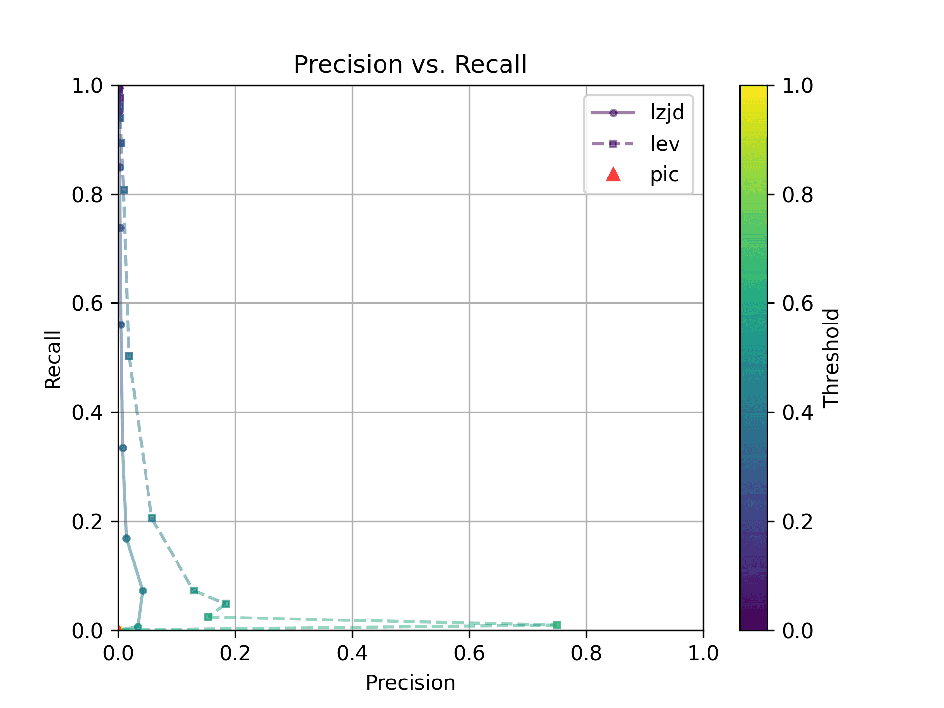
The first thing you might be wondering about in this graph is Where is PIC hashing? Well, it's there at (0, 0) if you look closely. The violin plot gives us a little more information about what is going on.
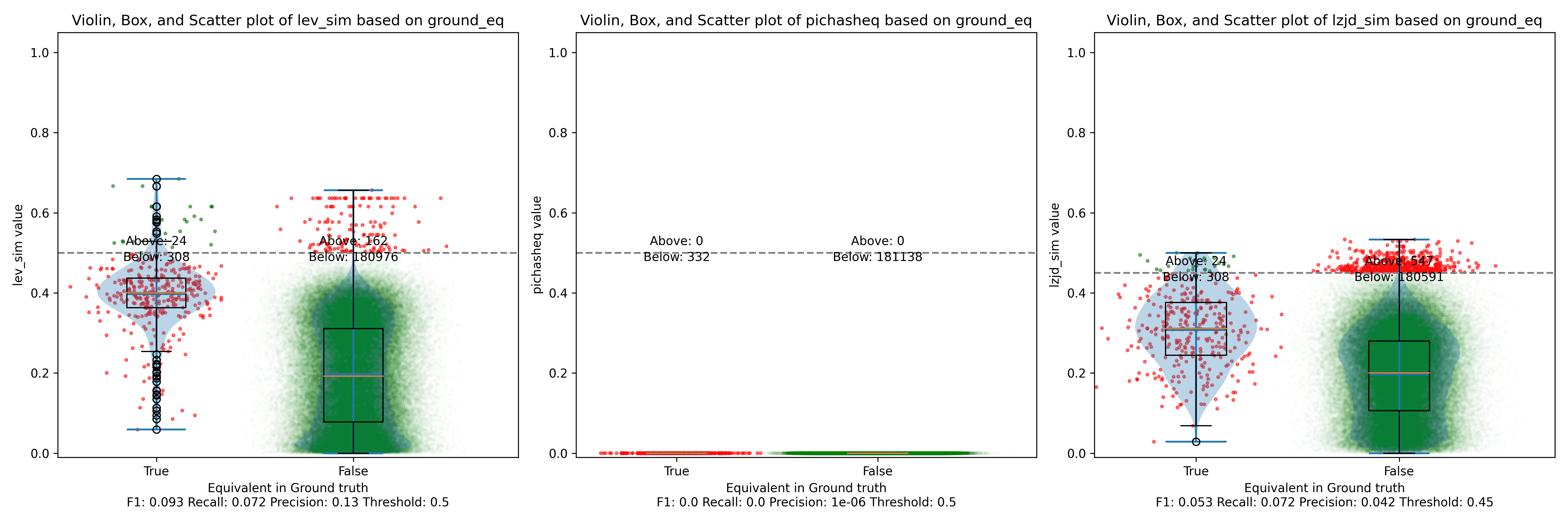
Here we can see that PIC hashing made no positive predictions. In other
words, none of the PIC hashes from the -O0 binary matched any of the PIC
hashes from the -O3 binary. I included this problem because I thought it
would be very challenging for PIC hashing, and I was right! But after some
discussion with Cory, we realized something fishy was going on. To achieve a
precision of 0.0, PIC hashing can't find any functions equivalent. That
includes trivially simple functions. If your function is just a ret
there's not much optimization to do.
Eventually, I guessed that the -O0 binary did not use the
-fomit-frame-pointer option, whereas all other optimization levels do. This
matters because this option changes the prologue and epilogue of every
function, which is why PIC hashing does so poorly here.
LEV and LZJD do slightly better again, achieving low (but non-zero) F1 scores. But to be fair, none of the techniques do very well here. It's a difficult problem.
-O2 and -O3
On the much easier extreme, let's look at -O2 and -O3.

Nice! PIC hashing does pretty well here, achieving a recall of 0.79 and a precision of 0.78. LEV and LZJD do about the same. However, the Precision vs. Recall graph for LEV shows a much more appealing trade-off line. LZJD's trade-off line is not nearly as appealing, as it's more horizontal.
You can start to see more of a difference between the distributions in the violin plots here in the LEV and LZJD panels.
I'll call this one a tie.
-O1 and -O2
I would also expect -O1 and -O2 to be fairly similar, but not as similar as
-O2 and -O3. Let's see:

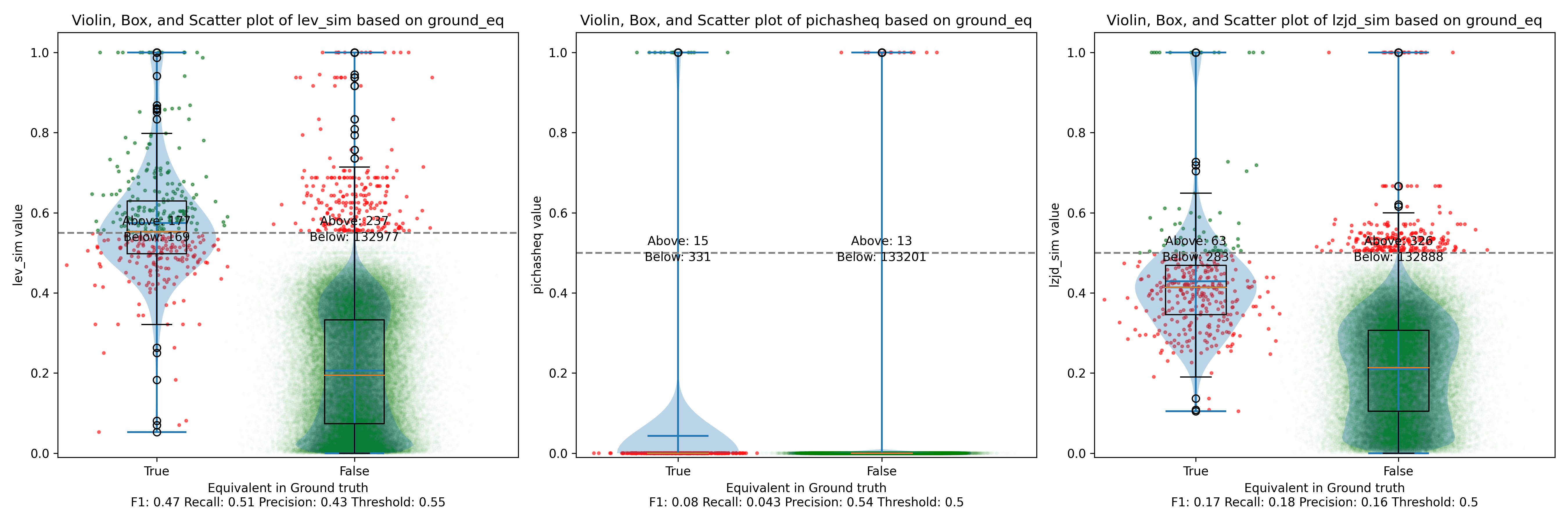
The Precision vs. Recall graph is very interesting. PIC hashing starts at a precision of 0.54 and a recall of 0.043. LEV in particular shoots straight up, indicating that by lowering the threshold, it is possible to increase recall substantially without losing much precision. A particularly attractive trade-off might be a precision of 0.43 and a recall of 0.51. This is the type of trade-off I was hoping for in fuzzy hashing.
Unfortunately, LZJD's trade-off line is again not nearly as appealing, as it curves in the wrong direction.
We'll say this is a pretty clear win for LEV.
-O1 and -O3
Finally, let's compare -O1 and -O3, which are different, but both have the
-fomit-frame-pointer option enabled by default.
These graphs look almost identical to comparing -O1 and -O2; I guess the
difference between -O2 and -O3 is really pretty minor. So it's again a win for LEV.
Experiment 2: Different openssl Versions
The final experiment I did was to compare various versions of openssl. This experiment was suggested by Cory, who thought it was reflective of typical malware RE scenarios. The idea is that the malware author released Malware 1.0, which you RE. Later, the malware changes a few things and releases Malware 1.1, and you want to detect which functions did not change so that you can avoid REing them again.
We looked at a few different versions of openssl:
| Version | Release Date | Months In Between |
|---|---|---|
| 1.0.2u | Dec 20, 2019 | N/A |
| 1.1.1 | Sep 11, 2018 | N/A |
| 1.1.1q | Oct 12, 2022 | 49 |
| 1.1.1v | Aug 1, 2023 | 9 |
| 1.1.1w | Sep 11, 2023 | 1 |
For each version, I compiled them using gcc -g -O2.
openssl 1.0 and 1.1 are different minor versions of openssl. As explained here,
Letter releases, such as 1.0.2a, exclusively contain bug and security fixes and no new features.
So, we would expect that openssl 1.0.2u is fairly different than any 1.1.1 version. And we would expect that in the same minor version, 1.1.1 would be similar to 1.1.1q, but would be more different than 1.1.1w.
Experiment 2a: openssl 1.0.2u vs 1.1.1w
As before, let's start with the most extreme comparison: 1.0.2u vs 1.1.1w.
Perhaps not too surprisingly, because the two binaries are quite different, all three techniques struggle. We'll say this is a three way tie.
Experiment 2b: openssl 1.1.1 vs 1.1.1w
Now let's look at the original 1.1.1 release from September 2018, and compare to the 1.1.1w bugfix release from September 2023. Although a lot of time has passed between the releases, the only differences should be bug and security fixes.

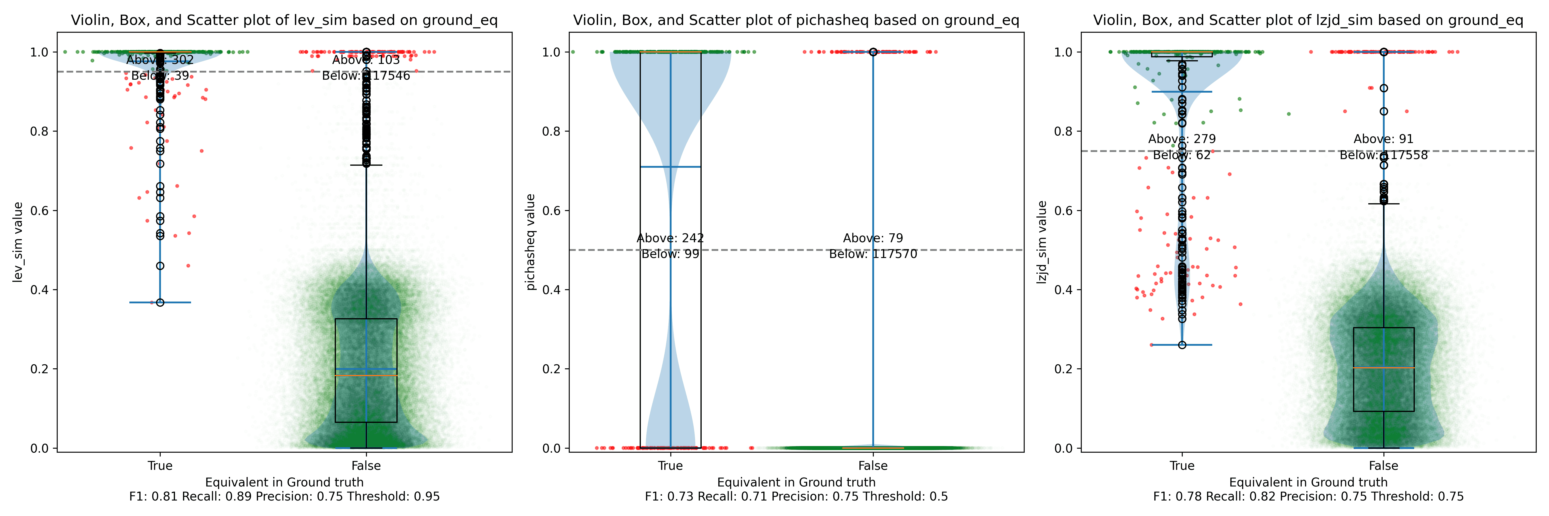
All three techniques do much better on this experiment, presumably because there are far fewer changes. PIC hashing achieves a precision of 0.75 and a recall of 0.71. LEV and LZJD go almost straight up, indicating an improvement in recall with minimal trade-off in precision. At roughly the same precision (0.75), LZJD achieves a recall of 0.82, and LEV improves it to 0.89.
LEV is the clear winner, with LZJD also showing a clear advantage over PIC.
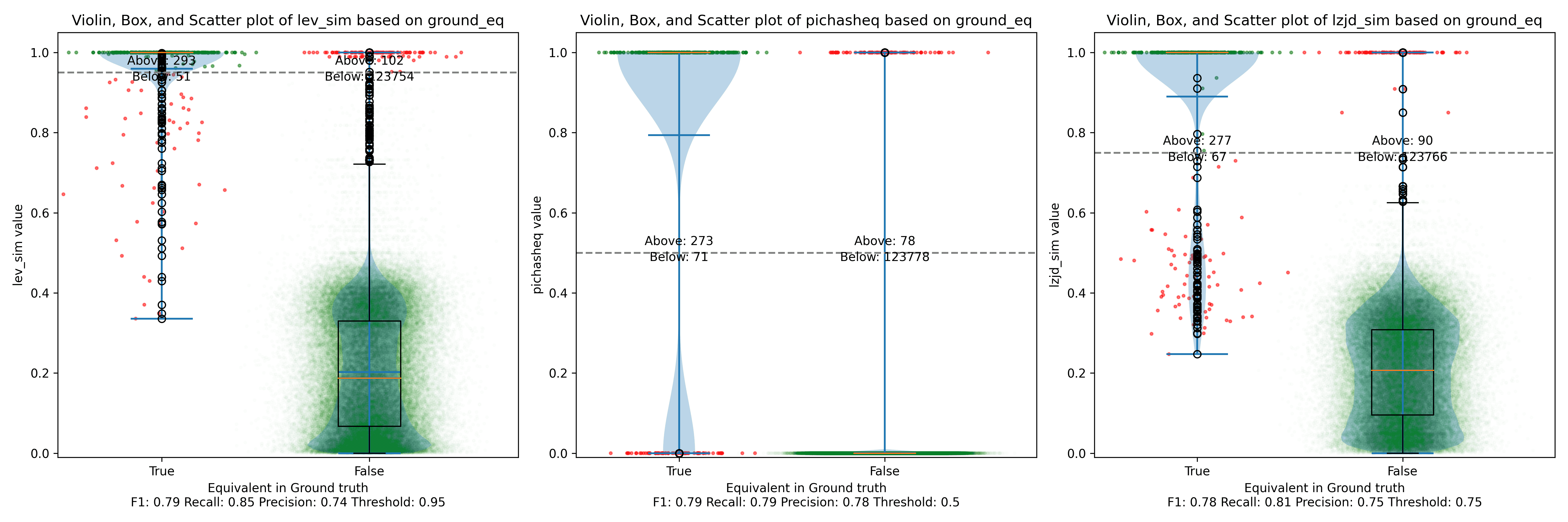
Experiment 2c: openssl 1.1.1q vs 1.1.1w
Let's continue looking at more similar releases. Now we'll compare 1.1.1q from July 2022 to 1.1.1w from September 2023.
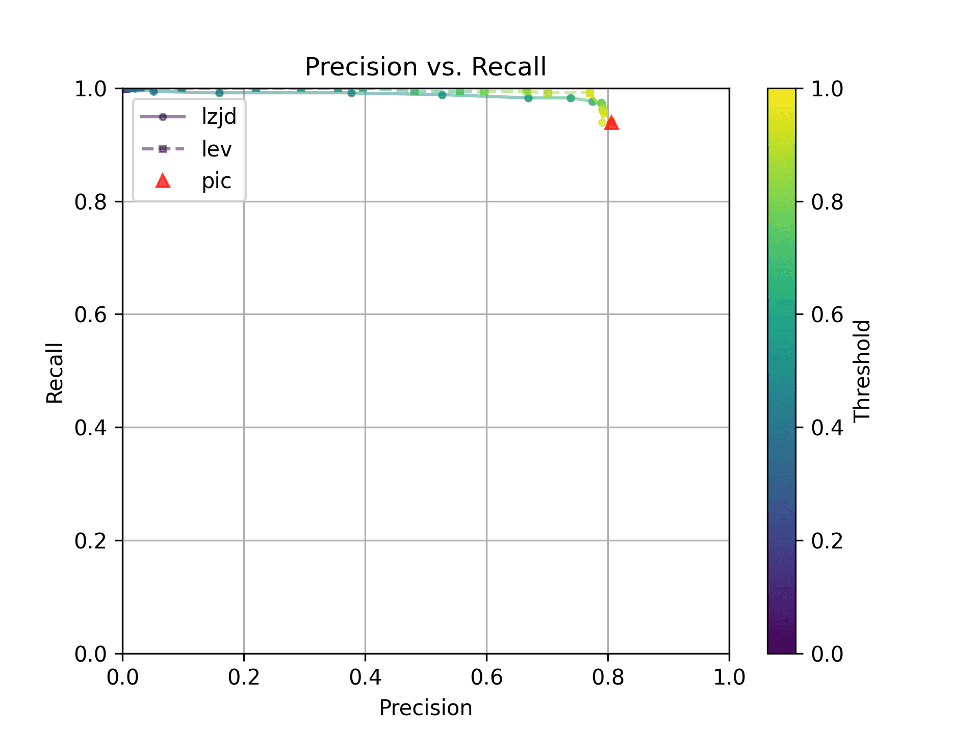
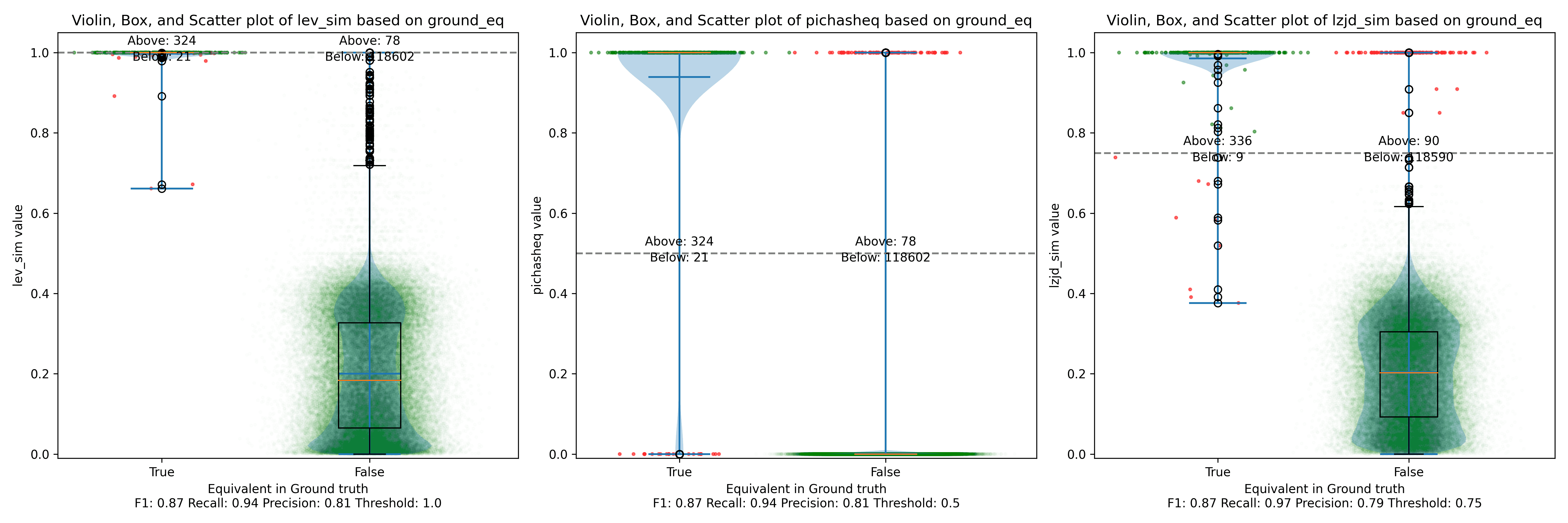
As can be seen in the Precision vs. Recall graph, PIC hashing starts at an impressive precision of 0.81 and a recall of 0.94. There simply isn't a lot of room for LZJD or LEV to make an improvement.
This is a three way tie.
Experiment 2d: openssl 1.1.1v vs 1.1.1w
Finally, we'll look at 1.1.1v and 1.1.1w, which were released only a month apart.
Unsurprisingly, PIC hashing does even better here, with a precision of 0.82 and a recall of 1.0 (after rounding)! Again, there's basically no room for LZJD or LEV to improve.
This is another three way tie.
Conclusion
Thresholds in Practice
We saw some scenarios where LEV and LZJD outperformed PIC hashing. But it's important to realize that we are conducting these experiments with ground truth, and we're using the ground truth to select the optimal threshold. You can see these thresholds listed at the bottom of each violin plot. Unfortunately, if you look carefully, you'll also notice that the optimal thresholds are not always the same. For example, the optimal threshold for LZJD in the "openssl 1.0.2u vs 1.1.1w" experiment was 0.95, but it was 0.75 in the "openssl 1.1.1q vs 1.1.1w" experiment.
In the real world, to use LZJD or LEV, you need to select a threshold. Unlike in these experiments, you could not select the optimal one, because you would have no way of knowing if your threshold was working well or not! If you choose a poor threshold, you might get substantially worse results than PIC hashing!
PIC Hashing is Pretty Good
I think we learned that PIC hashing is pretty good. It's not perfect, but it generally provides excellent precision. In theory, LZJD and LEV can perform better in terms of recall, which is nice, but in practice, it's not clear that they would because you would not know which threshold to use.
And although we didn't talk much about performance, PIC hashing is very fast. Although LZJD is much faster than LEV, it's still not nearly as fast as PIC.
Imagine you have a database of a million malware function samples, and you have a function that you want to look up in the database. For PIC hashing, this is just a standard database lookup, which can benefit from indexes and other precomputation techniques. For fuzzy hash approaches, we would need to invoke the similarity function a million times each time we wanted to do a database lookup.
There's a Limit to Syntactic Similarity
Remember that we used LEV to represent the optimal similarity based on the edit distance of instruction bytes. That LEV did not blow PIC out of the water is very telling, and suggests that there is a fundamental limit to how well syntactic similarity based on instruction bytes can perform. And surprisingly to me, PIC hashing appears to be pretty close to that limit. We saw a striking example of this limit when the frame pointer was accidentally omitted, and more generally, all syntactic techniques struggle when the differences become too great.
I wonder if any variants, like computing similarities over assembly code instead of executable code bytes, would perform any better.
Where Do We Go From Here?
There are of course other strategies for comparing similarity, such as incorporating semantic information. Many researchers have studied this. The general downside to semantic techniques is that they are substantially more expensive than syntactic techniques. But if you're willing to pay the price, you can get better results. Maybe in a future blog post we'll try one of these techniques out, such as the one my contemporary and friend Wesley Jin proposed in his dissertation.
While I was writing this blog post, Ghidra 11.0 also introduced BSim:
A major new feature called BSim has been added. BSim can find structurally similar functions in (potentially large) collections of binaries or object files. BSim is based on Ghidra's decompiler and can find matches across compilers used, architectures, and/or small changes to source code.
Another interesting question is whether we can use neural learning to help compute similarity. For example, we might be able to train a model to understand that omitting the frame pointer does not change the meaning of a function, and so shouldn't be counted as a difference.

Powered with by Gatsby 5.0