
OOAnalyzer is one of my favorite projects for a few reasons. The underlying problem is deceptively hard. If you look closely enough, OO executables have a lot of evidence in them. When you consider each piece in isolation, it can seem simple. But when you try to combine all of the evidence, you wind up with a combinatorial explosion of possibilities that is pruned by constraints in very complex ways. I also like it because it's a very practical problem. People actually use OOAnalyzer, despite all of its limitations—a testament to how even flawed solutions to hard problems can be valuable.
OOAnalyzer is a successor to an earlier project that predated me at SEI called ObjDigger. OOAnalyzer's big innovation was to use what we called "hypothetical reasoning" about ambiguous scenarios. In a nutshell, we often faced a choice between several possibilities. For example, class D inherits from class B, and we see class M in class D's vftable. We know that M is either a method of D or a method of B. We can't tell which one it is, but we can make a guess, and see if that leads to a contradiction. If it does, then we know our guess was wrong, and we can eliminate that possibility and try the others. This is a powerful technique that was partially enabled by our use of Prolog in OOAnalyzer, specifically Prolog's backtracking search.
That being said, OOAnalyzer's hypothetical reasoning is not perfect. One problem we encountered while developing OOAnalyzer was that there could be a long gap between a guess and when the contradiction is detected. Let's say we make a guess that eventually will cause a contradiction, but we must make 10 other boolean guesses before detecting the contradiction. At that point, Prolog would backtrack the guesses, starting with the most recent guess. Unfortunately, Prolog has no way of knowing that the actual cause was much further back, and it would waste time re-exploring models that were doomed to fail. Over time, we began to shape the rules in OOAnalyzer to avoid this problem. We ordered the rules so that any guess likely to lead to a contradiction would be detected immediately. This worked, but also limited our reasoning power.
Another problem with OOAnalyzer is how it decides on a final model. The final model is simply the first one that allows all guesses (uncertainties) to be resolved and does not lead to a contradiction. OOAnalyzer's guessing rules are ordered so that the more important ones are made earlier, when they have less chance of conflicting with a previous decision. But there is no guarantee that this model is the best one, or even close to it! Over time, I formed the opinion that OOAnalyzer is really an optimization problem. Our rules permit multiple models that could explain the evidence. But some are better than others. For example, many OO programs without vftables and vbtables can be explained by a model with no OO classes or methods. This is valid, but not very useful for the analyst.
Finally, OOAnalyzer involves a lot of constraints. For example, we might know that a method is either a constructor, real destructor, or deleting destructor. Obviously if we learn that the same method is not a destructor, it must be a constructor. Because we didn't use constraints in OOAnalyzer, we had to implement this type of logic manually. It works, but it's not elegant.
Over time, I've wondered how to better frame the OOAnalyzer problem, and recently I started exploring Answer Set Programming (ASP) as a potential answer. ASP is a form of declarative programming that is based on the stable model semantics of logic programming. It is designed to solve combinatorial search problems, and it has built-in support for constraints and optimization. ASP has several key features:
- It allows for declarative rules, like Prolog.
- It has built-in support for constraints.
1 { constructor(X); real_destructor(X); deleting_destructor(X) } 1means that exactly one of the three predicates must be true for any given X. - It has built-in support for optimization. We can assign weights to different models and ask the solver to find the global optimum, or the best solution found within a time limit.
In my spare time, I've been porting parts of OOAnalyzer to ASP here. I've been pleasantly surprised by how well it has worked so far. The code is much more concise and easier to read than the Prolog version. The constraints are much easier to express. For example, here's a rule that says if we see certain behavior (like installing vftables), we know that the method is a constructor or destructor:
% A method that writes a vftable/vbtable into its own this-pointer must be
% exactly one of: constructor, real destructor, or deleting destructor.
% Covers:
%   reasonConstructor (rules.pl:192) — elimination: only remaining candidate
%   reasonRealDestructor (rules.pl:388) — elimination: only remaining candidate
%   reasonDeletingDestructor (rules.pl:575) — elimination: only remaining candidate
%!trace_rule {"% is exactly one of constructor, real destructor, or deleting destructor", Method}
1 { constructor(Method) ; realDestructor(Method) ; deletingDestructor(Method) } 1 :-
    certainConstructorOrDestructor(Method).
Similarly, here's a rule saying that a method can only be one of a constructor, real destructor, or deleting destructor:
constructorDestructorKind(Method, constructor) :-
    constructor(Method).
constructorDestructorKind(Method, realDestructor) :-
    realDestructor(Method).
constructorDestructorKind(Method, deletingDestructor) :-
    deletingDestructor(Method).

% Covers:
%   insanityConstructorAndRealDestructor (insanity.pl:226)
%   insanityConstructorAndDeletingDestructor (insanity.pl:240)
%   reasonNOTConstructor_B (rules.pl:281) — realDestructor → notConstructor
%   reasonNOTConstructor_C (rules.pl:288) — deletingDestructor → notConstructor
%   reasonNOTRealDestructor_B (rules.pl:443) — constructor → notRealDestructor
%   reasonNOTRealDestructor_C (rules.pl:448) — deletingDestructor → notRealDestructor
%   reasonNOTDeletingDestructor_B (rules.pl:632) — constructor → notDeletingDestructor
%   reasonNOTDeletingDestructor_C (rules.pl:637) — realDestructor → notDeletingDestructor
%!trace_rule {"% has multiple constructor/destructor kinds", Method}
insanity(insanityMultipleConstructorDestructorKinds, (Method,Count)) :-
    method(Method),
    Count = #count { Kind : constructorDestructorKind(Method, Kind) },
    Count > 1.
As the comment above says, this rule covers about 8 different rules in OOAnalyzer. In ASP, we can express the same thing much more concisely.
OOAnalyzer-ASP can already read OOAnalyzer's facts format. You can see some examples of the results in the repository. Bear in mind that not all rules are ported yet.
One last thing I'll share is automatic explanations of models. I've been using the xclingo2 library to generate explanations for the ASP models. Even as OOAnalyzer's developer, it can be hard to understand how it reasons, because it could involve dozens of related conclusions. This is exacerbated in ASP because constraints and the optimization criteria are "silent". But even so, xclingo2 can generate detailed proof trees showing why a particular atom was included in the model. Here's an example of a proof tree for why a method is a constructor:
  |__4266400 is a constructor
  |  |__4266400 is a method;4266400 is a method because 4266176 calls it at this-offset 0
  |  |  |__thunk 4264566 resolves to 4266400
  |  |  |  |__thunk 4266400 resolves to 4266400
  |  |  |__4266176 is a method;4266176 is a method because it is a known constructor
  |  |  |  |__4266176 is a constructor;4266176 is exactly one of constructor, real destructor, or deleting destructor
  |  |  |  |  |__4266176 must be a constructor or destructor because it writes a vftable into its own this-pointer
  |  |  |  |  |  |__4266176 writes confirmed vftable 4290632 at offset 0
  |  |  |  |  |  |  |__4290632 is a confirmed vftable;4290632 is a confirmed vftable because RTTI says so
So is this the next generation OOAnalyzer? Theoretically, I think the answer is yes! But practically, it's unclear how well this is going to scale to real programs. One of the downsides to most ASP implementations is that they ground eagerly. Because executables can have a lot of evidence, it's possible this can lead to a combinatorial explosion in the number of ground rules. Because OOAnalyzer's rules involve negation and recursion in complex ways, it's hard to say how much of an issue this will be. We're able to find the optimal model on all of the toy OOAnalyzer programs, but that doesn't mean much. There are alternative approaches to ASP, like lazy grounding, but they are less mature. I'm hopeful that with cautious engineering, we can make this work on real programs, but only time will tell. In the meantime, I'm having fun exploring this new approach to the problem!
(Apologies in advance, this is probably going to be rambling.)
I spend a lot of time looking at various research artifacts. Yesterday, I was looking at several verification artifacts, and I was struck by how much impact small details like a Docker container can have. One of the projects I was using is STOKE. STOKE is a cool project, but the salient detail for this post is that it is an abandoned research project. The last commit was in December 2020. This is very common: Ph.D. student creates a project, maintains project, graduates, and then no longer maintains project. Despite that, STOKE has a Docker container, which makes using the project trivial.
In contrast, I was also attempting to run Psyche-C this week. Like STOKE, there's a fair bit of bitrot on the branch that contains the type-inference component. Unlike STOKE, Psyche-C does not have a Docker container. Part of this branch uses Haskell lts-5.1, which is from 2016! Trying to get this running was a nightmare, since modern versions of stack, GHC and cabal could not cope with such an old environment. I was eventually able to get it running by creating an Ubuntu focal docker image but it took me an entire day. I also created a HuggingFace space for it.
I have said it before, but I just love HuggingFace spaces for hosting research artifacts. It makes it almost effortless for others to try out your research. I wish more researchers would use them.
I think that the decompilation and reverse engineering research community could also significantly benefit from using HuggingFace spaces and generally making artifacts easier to use. I say this because there are many subtle details about reverse engineering research artifacts that can make them less usable in practice.
For example, I was recently reading DecompileBench, which is a good paper about benchmarking decompilers. In particular, they have a very clever method for testing whether a decompiled function is semantically equivalent to the original source code. In short, they compile the decompiled function in isolation and splice it into the original program, and do some testing to see if it behaves the same way. I've been thinking about this topic a lot recently, since I have been talking with some of my students about it. The problem is that if the binary is stripped, the decompiler can't refer to symbols by their original name, and thus the decompiled code can't reliably be linked back into the original program. (Ryan pointed out on Bluesky that this is possible in some cases.) DecompileBench ignores this problem and decompiled unstripped binaries. This is a problem, because decompilers are usually used on stripped binaries, and they generally perform significantly worse on them.
My goal is not to criticize DecompileBench; I think it's a nice paper. My point is that there are many subtle details like this that can make research artifacts less useful in practice. I've had my own share. As one example, the DIRT dataset was stripped using the wrong command, so that function names were still present in the binary, which is unrealistic. Fortunately, it turned out (surprisingly) that this did not significantly affect the results in that paper, but it could have.
I think part of the problem with these two examples is that it's hard to get close to the actual use case with these projects. In decompilation, the real use case is decompiling stripped binaries in the wild. But it's hard to run DIRTY on a new binary to see how well it works. I have found this to be a common problem in machine learning-based research. The straight-forward approach is to start with a dataset for which you have ground truth, and then train and test on that dataset. This often leads to preprocessing code that expects to have the ground truth information available. This is problematic when you want to perform inference on a new example when you don't have ground truth information, e.g., the primary use case of these technologies!
My overall message is that docker containers and HuggingFace spaces are great ways to make research artifacts easier to use. This is important in general, but it's also important to be able to get as close to the real use case as possible. If, for example, your technique only works for unstripped binaries and you forget to mention this in your paper, a docker container or space is going to make that very apparent.
I have a pretty hot take: the top-tier conferences should mandate that research artifacts be easy to use, e.g., via docker containers or HuggingFace spaces, on new examples, and that these artifacts should be considered as part of the submission. Having a separate, optional artifact evaluation process simply doesn't work. (The incentive for going through the artifact evaluation is a badge, which is essentially a sticker for grown-ups!) But if reviewers can actually try out the artifact on new examples, they can see how well it works in practice. This would significantly improve the quality of research artifacts in our community.


Systematic Testing of C++ Abstraction Recovery Systems by Iterative Compiler Model Refinement
I'm excited to announce that our paper, "Systematic Testing of C++ Abstraction Recovery Systems by Iterative Compiler Model Refinement", has been published at the 2025 Workshop on Software Understanding and Reverse Engineering (SURE)! SURE is a new workshop—more details below.
When I joined SEI, one of my first research projects was improving C++ abstraction recovery from binaries. This work led to the development of OOAnalyzer, a tool that combines practical reverse engineering with academic techniques like a Prolog-based reasoning engine.
Over time, users increasingly adopted OOAnalyze and ran it on video game executables that were much larger and more complex than the malware samples we had originally targeted. Perhaps unsurprisingly, running OOAnalyzer on these larger, more complex binaries often revealed problematic corner cases in OOAnalyzer's rules. As we learned about such problems, we would attempt to improve the rules to handle the new cases. Sometimes this was pretty easy; some of the problems were obvious in hindsight. But not always.
Eventually, I found that some rules were becoming so nuanced and complex that I was having trouble reasoning about them. I realized that I needed a more systematic way to test and refine OOAnalyzer's rules. This realization led to the work presented in this paper.
On one hand, I'm incredibly proud of this paper. To greatly simplify, we developed a way to model check the rules in OOAnalyzer. It's been incredibly effective at finding problems in OOAnalyzer's rules. We found 27 soundness issues in OOAnalyzer, and two in VirtAnalyzer, a competing C++ abstraction recovery system.
Unfortunately, the journey to publication for this paper has been long and bumpy. It is, admittedly, a fairly niche topic. But I also think it has some interesting ideas that could be applied more generally to other reverse engineering systems. In particular, I think that much of what we call "binary analysis" is actually "compiled executable analysis" in disguise. In other words, our binary analyses are often making (substantial!) assumptions about how compilers work, such as the calling conventions that are used, and without these assumptions they do not work. Our paper provides a systematic way to encode and refine these assumptions, and validate whether underlying analyses are correct under the assumptions. My hope is that in future work, we are able to demonstrate how to apply this overall approach to more traditional binary analyses. I personally think that static binary analysis without such reasonable simplifying assumptions is impractical, so we need more techniques like this to help analyze compiled executables.
Although I'm proud of the problems we discovered in OOAnalyzer, I'm also a bit disappointed in the practical impact. My hope was that when we found and fixed soundness problems in OOAnalyzer's rules, it would generally improve the performance of OOAnalyzer on real-world binaries. However, we found that in general this was not true. In fact, in some cases, fixing soundness problems actually made OOAnalyzer perform worse on real-world binaries! I think this highlights that there is a trade-off between soundness and accuracy in binary analysis. In order to be sound, the system can never make mistakes. We may need to make a rule more conservative, even if it almost never poses a problem in practice. However, in order to maximize accuracy, the system must optimize for the most common cases, even if it means that it will occasionally make mistakes.
SURE Workshop
SURE, the Workshop on Software Understanding and Reverse Engineering, is a new workshop colocated with ACM CCS this year. In addition to presenting our paper, I had the honor of participating in a panel on "Modern Software Understanding" alongside Fish Wang and Steffen Enders. The first SURE was a resounding success, and I'm eager to see how it evolves in the coming years!
🎉 New Research Published at DIMVA 2025
I'm excited to announce that "Quantifying and Mitigating the Impact of Obfuscations on Machine-Learning-Based Decompilation Improvement" has been published at the 2025 Conference on Detection of Intrusions and Malware & Vulnerability Assessment (DIMVA 2025)!
The Research Team
This work was primarily conducted by Deniz Bölöni-Turgut—a bright undergraduate at Cornell University—as part of the REU in Software Engineering (REUSE) program at CMU. She was supervised by Luke Dramko from our research group.
What We Investigated
This paper tackles an important question in the evolving landscape of AI-powered reverse engineering: How do code obfuscations impact the effectiveness of these ML-based approaches? In the real world, adversaries often employ obfuscation techniques to make their code harder to analyze by reverse engineers. Although these obfuscation techniques were not designed with machine learning in mind, they can significantly modify the code, which raises the question of whether they could hinder the performance of ML models, which are currently trained on unobfuscated code.
Key Findings
Our research provides important quantitative insights into how obfuscations affect ML-based decompilation:
-
Obfuscations do negatively impact ML models: We demonstrated that semantics-preserving transformations that obscure program functionality significantly reduce the accuracy of machine learning-based decompilation tools.
-
Training on obfuscated code helps: Our experiments show that training models on obfuscated code can partially recover the lost accuracy, making the tools more resilient to obfuscation techniques.
-
Consistent results across multiple models: We validated our findings across three different state-of-the-art models from the literature—DIRTY, HexT5, and VarBERT—suggesting that our findings generalize.
-
Practical implications for malware analysis: Since obfuscations are commonly used in malware, these findings are directly applicable to improving real-world binary analysis scenarios.
This work represents an important step forward in making ML-based decompilation tools more resilient against the obfuscation techniques commonly encountered in real-world binary analysis scenarios. As the field continues to evolve, understanding these vulnerabilities and developing robust solutions will be crucial for maintaining the effectiveness of AI-powered security tools.
Read More
Want to know more? Download the complete paper.
🎉 New Research Published at DSN 2025
I'm excited to announce that "A Human Study of Automatically Generated Decompiler Annotations" has been published at the 2025 IEEE/IFIP International Conference on Dependable Systems and Networks (DSN 2025)!
The Research Team
This work represents the culmination of Jeremy Lacomis's Ph.D. research, alongside our fantastic collaborators:
- Vanderbilt University: Yuwei Yang, Skyler Grandel, and Kevin Leach
- Carnegie Mellon University: Bogdan Vasilescu and Claire Le Goues
What We Studied
This paper investigates a critical question in reverse engineering: Do automatically generated variable names and type annotations actually help human analysts understand decompiled code?
Our study built upon DIRTY, our machine learning system that automatically generates meaningful variable names and type information for decompiled binaries. While DIRTY showed promising technical results, we wanted to understand its real-world impact on human reverse engineers.
Key Findings
- Surprisingly, the annotations did not significantly improve participants' task completion speed or accuracy
- This challenges assumptions about the direct correlation between code readability and task performance
- Participants preferred code with annotations over plain decompiled output
Read More
Interested in the full methodology and detailed results? Download the complete paper to dive deeper into our human study design, statistical analysis, and implications for future decompilation tools.
Can existing neural decompiler artifacts be used to run on a new example? Here are some notes on the current state of the art. I assign each decompiler a score from 0 to 10 based on how easy it is to use the publicly available artifacts to run on a new example.
SLaDe: 2/10
SLaDe has a publicly released replication artifact but there are several problems that prevent it from being used on new examples:
- The models are trained on assembly code produced from compilers rather than disassemblers. This is probably minor.
- More problematically, SLaDe uses IO testcases during beam search to help detect the best candidate. It can be used without these, but the results will be worse. SLaDe does not contain a mechanism for producing testcases for new examples.
Below is a quote from a private conversation with the author:
You are right that IO are somehow used to select in the beam search, in the sense that we report pass@5. They are not strictly required to get the outputs though.
The link you sent is for the program synthesis dataset. In this one, IO generation was programmatic but still kind of manual, I don't think it would be feasible to automatically generate the props file in the general case. For the Github functions, we have a separate repo that automatically generates IO tests, but those are randomly generated and the quality depends on each case. If I had to redo now, I would ask an LLM to generate unit tests! I can give you access to the private repo we used to automatically generate the IO examples for the general case if you wish, but now I'd do it with LLMs rather than randomly.
LLM4Decompile: 9/10
LLM4Decompile has published model files on HuggingFace that can easily be used to run on new examples. I created a few HuggingFace Spaces for testing.
resym: 2/10
resym has a publicly released replication artifact. Unfortunately, as of February 2025, the artifact is missing the "prolog-based inference system for struct layout recovery" which is the key contribution of the paper. Thus it is not possible to run resym on new examples.
DeGPT: 8/10
DeGPT has a publicly released GitHub repository. I'm largely going on memory, but I used it previously on new examples and it was relatively easy to use. I did have to file a few PRs though.
Imagine that you reverse engineered a piece of malware in pain-staking detail, only to find that the malware author created a slightly modified version of the malware the next day. You wouldn't want to redo all your hard work. One way to avoid this is to use code comparison techniques to try to identify pairs of functions in the old and new version that are "the same" (which I put in quotes because it's a bit of a nebulous concept, as we'll see).
There are several tools to help in such situations. A very popular (formerly) commercial tool is zynamics' bindiff, which is now owned by Google and free. CMU SEI's Pharos also includes a code comparison utility called fn2hash, which is the subject of this blog post.
Background
Exact Hashing
fn2hash employs several types of hashing, with the most commonly used one called PIC hashing, where PIC stands for Position Independent Code. To see why PIC hashing is important, we'll actually start by looking at a naive precursor to PIC hashing, which is to simply hash the instruction bytes of a function. We'll call this exact hashing.
Let's look at an example. I compiled this simple program
oo.cpp with
g++. Here's the beginning of the assembly code for the function myfunc
(full
code):
Assembly code and bytes from oo.gcc
;;;;;;;;;;;;;;;;;;;;;;;;;;;;;;;;;;;;;;;;;;;;;;;;;;;;;;;;;;;;;;;;;;;;;;;;;;;;;;;;;;;;;;;;;;;;;;;;;;;;;;;;;;;;;;;;;;;;;;;;
;;; function 0x00401200 "myfunc()"
;;; mangled name is "_Z6myfuncv"
;;; reasons for function: referenced by symbol table

;; predecessor:  from instruction 0x004010f4 from basic block 0x004010f0
0x00401200: 41 56                      00 push     r140x00401202: bf 60 00 00 00            -08 mov      edi, 0x00000060<96>
0x00401207: 41 55                     -08 push     r13
0x00401209: 41 54                     -10 push     r12
0x0040120b: 55                        -18 push     rbp
0x0040120c: 48 83 ec 08               -20 sub      rsp, 8
0x00401210: e8 bb fe ff ff            -28 call     function 0x004010d0 "operator new(unsigned long)@plt"
Exact Bytes
In the first highlighted line, you can see that the first instruction is a
push r14, which is encoded by the instruction bytes 41 56. If we collect the
encoded instruction bytes for every instruction in the function, we get:
Exact bytes in oo.gcc
4156BF6000000041554154554883EC08E8BBFEFFFFBF6000000048C700F02040004889C548C7401010214000C740582A000000E898FEFFFFBF1000000048C700F02040004989C448C7401010214000C740582A000000E875FEFFFFBA0D000000BE48204000BF80404000C74008000000004989C5C6400C0048C700D8204000E82CFEFFFF488B05F52D0000488B40E84C8BB0704140004D85F60F842803000041807E38000F84160200004C89F7E898FBFFFF498B06BE0A000000488B4030483DD01540000F84CFFDFFFF4C89F7FFD00FBEF0E9C2FDFFFF410FBE7643BF80404000E827FEFFFF4889C7E8FFFDFFFF488B4500488B00483DE01740000F85AC0200004889EFFFD0488B4500488B4008483D601640000F84A0FDFFFFBA0D000000BE3A204000BF80404000E8C8FDFFFF488B05912D0000488B40E84C8BB0704140004D85F60F84C402000041807E38000F84820100004C89F7E8C8FBFFFF498B06BE0A000000488B4030483DD01540000F8463FEFFFF4C89F7FFD00FBEF0E956FEFFFF410FBE7643BF80404000E8C3FDFFFF4889C7E89BFDFFFF488B4500488B4008483D601640000F85600200004889EFFFD0E9E7FDFFFFBA0D000000BE1E204000BF80404000E863FDFFFF488B052C2D0000488B40E84C8BB0704140004D85F60F845F02000041807E38000F847D0100004C89F7E868FBFFFF498B06BE0A000000488B4030483DD01540000F8468FEFFFF4C89F7FFD00FBEF0E95BFEFFFF410FBE7643BF80404000E85EFDFFFF4889C7E836FDFFFF488B4510488D7D10488B4008483DE01540000F8506020000FFD0498B0424488B00483DE01740000F8449FEFFFFBA0D000000BE10204000BF80404000E8FAFCFFFF488B05C32C0000488B40E84C8BB0704140004D85F60F84F601000041807E38000F84440100004C89F7E838FBFFFF498B06BE0A000000488B4030483DD01540000F84A1FEFFFF4C89F7FFD00FBEF0E994FEFFFF410FBE7643BF80404000E8F5FCFFFF4889C7E8CDFCFFFF498B0424488B00483DE01740000F85B70100004C89E7FFD0E990FEFFFFBA0D000000BE3A204000BF80404000E896FCFFFF488B055F2C0000488B40E84C8BB0704140004D85F60F8492010000E864FAFFFF0F1F400041807E38000F84100100004C89F7E808FBFFFF498B06BE0A000000488B4030483DD01540000F84D5FEFFFF4C89F7FFD00FBEF0E9C8FEFFFF410FBE7643BF80404000E891FCFFFF4889C7E869FCFFFF4889EFBE60000000E8FC0300004C89E7BE10000000E8EF0300004883C4084C89EFBE100000005D415C415D415EE9D7030000We call this sequence the exact bytes of the function. We can hash these bytes to get an exact hash, 62CE2E852A685A8971AF291244A1283A.
Short-comings of Exact Hashing
The highlighted call at address 0x401210 is a relative call, which means that
the target is specified as an offset from the current instruction (well,
technically the next instruction). If you look at the instruction bytes for this
instruction, it includes the bytes bb fe ff ff, which is 0xfffffebb in little
endian form; interpreted as a signed integer value, this is -325. If we take
the address of the next instruction (0x401210 + 5 == 0x401215) and then add -325
to it, we get 0x4010d0, which is the address of operator new, the target of
the call. Yay. So now we know that bb fe ff ff is an offset from the next
instruction. Such offsets are called relative offsets because they are
relative to the address of the next instruction.
I created a slightly modified
program (oo2.gcc) by
adding an empty, unused function before myfunc. You can find the disassembly
of myfunc for this executable
here.
If we take the exact hash of myfunc in this new executable, we get
05718F65D9AA5176682C6C2D5404CA8D. Wait, that's different than the hash for
myfunc in the first executable, 62CE2E852A685A8971AF291244A1283A. What
happened? Let's look at the disassembly.
Assembly code and bytes from oo2.gcc
;;;;;;;;;;;;;;;;;;;;;;;;;;;;;;;;;;;;;;;;;;;;;;;;;;;;;;;;;;;;;;;;;;;;;;;;;;;;;;;;;;;;;;;;;;;;;;;;;;;;;;;;;;;;;;;;;;;;;;;;
;;; function 0x00401210 "myfunc()"

;; predecessor:  from instruction 0x004010f4 from basic block 0x004010f0
0x00401210: 41 56                      00 push     r14
0x00401212: bf 60 00 00 00            -08 mov      edi, 0x00000060<96>
0x00401217: 41 55                     -08 push     r13
0x00401219: 41 54                     -10 push     r12
0x0040121b: 55                        -18 push     rbp
0x0040121c: 48 83 ec 08               -20 sub      rsp, 8
0x00401220: e8 ab fe ff ff            -28 call     function 0x004010d0 "operator new(unsigned long)@plt"
Notice that myfunc moved from 0x401200 to 0x401210, which also moved the
address of the call instruction from 0x401210 to 0x401220. Because the call
target is specified as an offset from the (next) instruction's address, which
changed by 0x10 == 16, the offset bytes for the call changed from bb fe ff ff
(-325) to ab fe ff ff (-341 == -325 - 16). These changes modify the exact
bytes to:
Exact bytes in oo2.gcc
4156BF6000000041554154554883EC08E8ABFEFFFFBF6000000048C700F02040004889C548C7401010214000C740582A000000E888FEFFFFBF1000000048C700F02040004989C448C7401010214000C740582A000000E865FEFFFFBA0D000000BE48204000BF80404000C74008000000004989C5C6400C0048C700D8204000E81CFEFFFF488B05E52D0000488B40E84C8BB0704140004D85F60F842803000041807E38000F84160200004C89F7E888FBFFFF498B06BE0A000000488B4030483DE01540000F84CFFDFFFF4C89F7FFD00FBEF0E9C2FDFFFF410FBE7643BF80404000E817FEFFFF4889C7E8EFFDFFFF488B4500488B00483DF01740000F85AC0200004889EFFFD0488B4500488B4008483D701640000F84A0FDFFFFBA0D000000BE3A204000BF80404000E8B8FDFFFF488B05812D0000488B40E84C8BB0704140004D85F60F84C402000041807E38000F84820100004C89F7E8B8FBFFFF498B06BE0A000000488B4030483DE01540000F8463FEFFFF4C89F7FFD00FBEF0E956FEFFFF410FBE7643BF80404000E8B3FDFFFF4889C7E88BFDFFFF488B4500488B4008483D701640000F85600200004889EFFFD0E9E7FDFFFFBA0D000000BE1E204000BF80404000E853FDFFFF488B051C2D0000488B40E84C8BB0704140004D85F60F845F02000041807E38000F847D0100004C89F7E858FBFFFF498B06BE0A000000488B4030483DE01540000F8468FEFFFF4C89F7FFD00FBEF0E95BFEFFFF410FBE7643BF80404000E84EFDFFFF4889C7E826FDFFFF488B4510488D7D10488B4008483DF01540000F8506020000FFD0498B0424488B00483DF01740000F8449FEFFFFBA0D000000BE10204000BF80404000E8EAFCFFFF488B05B32C0000488B40E84C8BB0704140004D85F60F84F601000041807E38000F84440100004C89F7E828FBFFFF498B06BE0A000000488B4030483DE01540000F84A1FEFFFF4C89F7FFD00FBEF0E994FEFFFF410FBE7643BF80404000E8E5FCFFFF4889C7E8BDFCFFFF498B0424488B00483DF01740000F85B70100004C89E7FFD0E990FEFFFFBA0D000000BE3A204000BF80404000E886FCFFFF488B054F2C0000488B40E84C8BB0704140004D85F60F8492010000E854FAFFFF0F1F400041807E38000F84100100004C89F7E8F8FAFFFF498B06BE0A000000488B4030483DE01540000F84D5FEFFFF4C89F7FFD00FBEF0E9C8FEFFFF410FBE7643BF80404000E881FCFFFF4889C7E859FCFFFF4889EFBE60000000E8FC0300004C89E7BE10000000E8EF0300004883C4084C89EFBE100000005D415C415D415EE9D7030000You can look through that and see the differences by eyeballing it. Just kidding! Here's a visual comparison. Red represents bytes that are only in oo.gcc, and green represents bytes in oo2.gcc. The differences are small because the offset is only changing by 0x10, but this is enough to break exact hashing.
Difference between exact bytes in oo.gcc and oo2.gcc
4156BF6000000041554154554883EC08E8BBABFEFFFFBF6000000048C700F02040004889C548C7401010214000C740582A000000E89888FEFFFFBF1000000048C700F02040004989C448C7401010214000C740582A000000E87565FEFFFFBA0D000000BE48204000BF80404000C74008000000004989C5C6400C0048C700D8204000E82C1CFEFFFF488B05F5E52D0000488B40E84C8BB0704140004D85F60F842803000041807E38000F84160200004C89F7E89888FBFFFF498B06BE0A000000488B4030483DD0E01540000F84CFFDFFFF4C89F7FFD00FBEF0E9C2FDFFFF410FBE7643BF80404000E82717FEFFFF4889C7E8FFEFFDFFFF488B4500488B00483DE0F01740000F85AC0200004889EFFFD0488B4500488B4008483D60701640000F84A0FDFFFFBA0D000000BE3A204000BF80404000E8C8B8FDFFFF488B0591812D0000488B40E84C8BB0704140004D85F60F84C402000041807E38000F84820100004C89F7E8C8B8FBFFFF498B06BE0A000000488B4030483DD0E01540000F8463FEFFFF4C89F7FFD00FBEF0E956FEFFFF410FBE7643BF80404000E8C3B3FDFFFF4889C7E89B8BFDFFFF488B4500488B4008483D60701640000F85600200004889EFFFD0E9E7FDFFFFBA0D000000BE1E204000BF80404000E86353FDFFFF488B052C1C2D0000488B40E84C8BB0704140004D85F60F845F02000041807E38000F847D0100004C89F7E86858FBFFFF498B06BE0A000000488B4030483DD0E01540000F8468FEFFFF4C89F7FFD00FBEF0E95BFEFFFF410FBE7643BF80404000E85E4EFDFFFF4889C7E83626FDFFFF488B4510488D7D10488B4008483DE0F01540000F8506020000FFD0498B0424488B00483DE0F01740000F8449FEFFFFBA0D000000BE10204000BF80404000E8FAEAFCFFFF488B05C3B32C0000488B40E84C8BB0704140004D85F60F84F601000041807E38000F84440100004C89F7E83828FBFFFF498B06BE0A000000488B4030483DD0E01540000F84A1FEFFFF4C89F7FFD00FBEF0E994FEFFFF410FBE7643BF80404000E8F5E5FCFFFF4889C7E8CDBDFCFFFF498B0424488B00483DE0F01740000F85B70100004C89E7FFD0E990FEFFFFBA0D000000BE3A204000BF80404000E89686FCFFFF488B055F4F2C0000488B40E84C8BB0704140004D85F60F8492010000E86454FAFFFF0F1F400041807E38000F84100100004C89F7E808FBF8FAFFFF498B06BE0A000000488B4030483DD0E01540000F84D5FEFFFF4C89F7FFD00FBEF0E9C8FEFFFF410FBE7643BF80404000E89181FCFFFF4889C7E86959FCFFFF4889EFBE60000000E8FC0300004C89E7BE10000000E8EF0300004883C4084C89EFBE100000005D415C415D415EE9D7030000
PIC Hashing
This problem is the motivation for few different types of hashing that we'll
talk about in this blog post, including PIC hashing and fuzzy hashing. The
PIC in PIC hashing stands for Position Independent Code. At a high level,
the goal of PIC hashing is to compute a hash or signature of code, but do so in
a way that relocating the code will not change the hash. This is important
because, as we just saw, modifying a program often results in small changes to
addresses and offsets and we don't want these changes to modify the hash!. The
intuition behind PIC hashing is very straight-forward: identify offsets and
addresses that are likely to change if the program is recompiled, such as bb fe ff ff,
and simply set them to zero before hashing the bytes. That way if they
change because the function is relocated, the function's PIC hash won't change.
The following visual diff shows the differences between the exact bytes and the
PIC bytes on myfunc in oo.gcc. Red represents bytes that are only in the PIC
bytes, and green represents the exact bytes. As expected, the first
change we can see is the byte sequence bb fe ff ff, which is changed to zeros.
Byte difference between PIC bytes (red) and exact bytes (green)
4156BF6000000041554154554883EC08E800000000BBFEFFFFBF6000000048C700000000F02040004889C548C7401000000010214000C740582A000000E80000000098FEFFFFBF1000000048C700000000F02040004989C448C7401000000010214000C740582A000000E80000000075FEFFFFBA0D000000BE00000048204000BF00000080404000C74008000000004989C5C6400C0048C700000000D8204000E8000000002CFEFFFF488B050000F52D0000488B40E84C8BB0000000704140004D85F60F842803000041807E38000F84160200004C89F7E80000000098FBFFFF498B06BE0A000000488B4030483D000000D01540000F84CFFDFFFF4C89F7FFD00FBEF0E9C2FDFFFF410FBE7643BF00000080404000E80000000027FEFFFF4889C7E800000000FFFDFFFF488B4500488B00483D000000E01740000F85AC0200004889EFFFD0488B4500488B4008483D000000601640000F84A0FDFFFFBA0D000000BE0000003A204000BF00000080404000E800000000C8FDFFFF488B050000912D0000488B40E84C8BB0000000704140004D85F60F84C402000041807E38000F84820100004C89F7E800000000C8FBFFFF498B06BE0A000000488B4030483D000000D01540000F8463FEFFFF4C89F7FFD00FBEF0E956FEFFFF410FBE7643BF00000080404000E800000000C3FDFFFF4889C7E8000000009BFDFFFF488B4500488B4008483D000000601640000F85600200004889EFFFD0E9E7FDFFFFBA0D000000BE0000001E204000BF00000080404000E80000000063FDFFFF488B0500002C2D0000488B40E84C8BB0000000704140004D85F60F845F02000041807E38000F847D0100004C89F7E80000000068FBFFFF498B06BE0A000000488B4030483D000000D01540000F8468FEFFFF4C89F7FFD00FBEF0E95BFEFFFF410FBE7643BF00000080404000E8000000005EFDFFFF4889C7E80000000036FDFFFF488B4510488D7D10488B4008483D000000E01540000F8506020000FFD0498B0424488B00483D000000E01740000F8449FEFFFFBA0D000000BE00000010204000BF00000080404000E800000000FAFCFFFF488B050000C32C0000488B40E84C8BB0000000704140004D85F60F84F601000041807E38000F84440100004C89F7E80000000038FBFFFF498B06BE0A000000488B4030483D000000D01540000F84A1FEFFFF4C89F7FFD00FBEF0E994FEFFFF410FBE7643BF00000080404000E800000000F5FCFFFF4889C7E800000000CDFCFFFF498B0424488B00483D000000E01740000F85B70100004C89E7FFD0E990FEFFFFBA0D000000BE0000003A204000BF00000080404000E80000000096FCFFFF488B0500005F2C0000488B40E84C8BB0000000704140004D85F60F8492010000E80000000064FAFFFF0F1F400041807E38000F84100100004C89F7E80000000008FBFFFF498B06BE0A000000488B4030483D000000D01540000F84D5FEFFFF4C89F7FFD00FBEF0E9C8FEFFFF410FBE7643BF00000080404000E80000000091FCFFFF4889C7E80000000069FCFFFF4889EFBE60000000E80000FC0300004C89E7BE10000000E80000EF0300004883C4084C89EFBE100000005D415C415D415EE90000D7030000
If we hash the PIC bytes, we get the PIC hash
EA4256ECB85EDCF3F1515EACFA734E17. And, as we would hope, we get the same PIC
hash for myfunc in the slightly modified oo2.gcc.
Evaluating the Accuracy of PIC Hashing
The primary motivation behind PIC hashing is to detect identical code that is moved to a different location. But what if two pieces of code are compiled with different compilers or different compiler flags? What if two functions are very similar, but one has a line of code removed? Because these changes would modify the non-offset bytes that are used in the PIC hash, it would change the PIC hash of the code. Since we know that PIC hashing will not always work, in this section we'll discuss how we can measure the performance of PIC hashing and compare it to other code comparison techniques.
Before we can define the accuracy of any code comparison technique, we'll need some ground truth that tells us which functions are equivalent. For this blog post, we'll use compiler debug symbols to map function addresses to their names. This will provide us with a ground truth set of functions and their names. For the purposes of this blog post, and general expediency, we'll assume that if two functions have the same name, they are "the same". (This obviously is not true in general!)
Confusion Matrices
So, let's say we have two similar executables, and we want to evaluate how well PIC hashing can identify equivalent functions across both executables. We'll start by considering all possible pairs of functions, where each pair contains a function from each executable. If we're being mathy, this is called the cartesian product (between the functions in the first executable and the functions in the second executable). For each function pair, we'll use the ground truth to determine if the functions are the same by seeing if they have the same name. Then we'll use PIC hashing to predict whether the functions are the same by computing their hashes and seeing if they are identical. There are two outcomes for each determination, so there are four possibilities in total:
- True Positive (TP): PIC hashing correctly predicted the functions are equivalent.
- True Negative (TN): PIC hashing correctly predicted the functions are different.
- False Positive (FP): PIC hashing incorrectly predicted the functions are equivalent, but they are not.
- False Negative (FN): PIC hashing incorrectly predicted the functions are different, but they are equivalent.
To make it a little easier to interpret, we color the good outcomes green and the bad outcomes red.
We can represent these in what is called a confusion matrix:
| Hashing says same | Hashing says different | |
|---|---|---|
| Ground truth says same | TP | FN |
| Ground truth says different | FP | TN |
For example, here is a confusion matrix from an experiment where I use PIC hashing to compare openssl versions 1.1.1w and 1.1.1v when they are both compiled in the same manner. These two versions of openssl are very similar, so we would expect that PIC hashing would do well because a lot of functions will be identical but shifted to different addresses. And, indeed, it does:
| Hashing says same | Hashing says different | |
|---|---|---|
| Ground truth says same | 344 | 1 |
| Ground truth says different | 78 | 118,602 |
Metrics: Accuracy, Precision, and Recall
So when does PIC hashing work well, and when does it not? In order to answer these questions, we're going to need an easier way to evaluate the quality of a confusion matrix as a single number. At first glance, accuracy seems like the most natural metric, which tell us: How many pairs did hashing predict correctly? This is equal to
For the above example, PIC hashing achieved an accuracy of
99.9% accuracy. Pretty good, right?
But if you look closely, there's a subtle problem. Most function pairs are not equivalent. According to the ground truth, there are equivalent function pairs, and non-equivalent function pairs. So, if we just guessed that all function pairs were non-equivalent, we would still be right of the time. Since accuracy weights all function pairs equally, it is not the best metric here.
Instead, we want a metric that emphasizes positive results, which in this case are equivalent function pairs. This is consistent with our goal in reverse engineering, because knowing that two functions are equivalent allows a reverse engineer to transfer knowledge from one executable to another and save time!
Three metrics that focus more on positive cases (i.e., equivalent functions) are precision, recall, and F1 score:
- Precision: Of the function pairs hashing declared equivalent, how many were actually equivalent? This is equal to .
- Recall: Of the equivalent function pairs, how many did hashing correctly declare as equivalent? This is equal to .
- F1 score: This is a single metric that reflects both the Precision and Recall. Specifically, it is the harmonic mean of the Precision and Recall, or . Compared to the arithmetic mean, the harmonic mean is more sensitive to low values. This means that if either Precision or Recall is low, the F1 score will also be low.
So, looking at the above example, we can compute the precision, recall, and F1 score. The precision is , the recall is , and the F1 score is . So, PIC hashing is able to identify 81% of equivalent function pairs, and when it does declare a pair is equivalent, it is correct 99.7% of the time. This corresponds to a F1 score of 0.89 out of 1.0, which is pretty good!
Now, you might be wondering how well PIC hashing performs when the differences between executables are larger.
Let's look at another experiment. In this one, I compare an openssl executable compiled with gcc to one compiled with clang. Because gcc and clang generate assembly code differently, we would expect there to be a lot more differences.
Here is a confusion matrix from this experiment:
| Hashing says same | Hashing says different | |
|---|---|---|
| Ground truth says same | 23 | 301 |
| Ground truth says different | 31 | 117,635 |
In this example, PIC hashing achieved a recall of , and a precision of . So, hashing is only able to identify 7% of equivalent function pairs, but when it does declare a pair is equivalent, it is correct 43% of the time. This corresponds to a F1 score of 0.12 out of 1.0, which is pretty bad. Imagine that you spent hours reverse engineering the 324 functions in one of the executables, only to find that PIC hashing was only able to identify 23 of them in the other executable, so you would be forced to needlessly reverse engineer the other functions from scratch. That would be pretty frustrating! Can we do better?
The Great Fuzzy Hashing Debate
There's a very different type of hashing called fuzzy hashing. Like regular
hashing, there is a hash function that reads a sequence of bytes and produces a hash.
Unlike regular hashing, though, you don't compare fuzzy hashes with equality.
Instead, there is a similarity function which takes two fuzzy hashes as input,
and returns a number between 0 and 1, where 0 means completely dissimilar, and 1
means completely similar.
My colleague, Cory Cohen, and I, actually debated whether there is utility in applying fuzzy hashes to instruction bytes, and our debate motivated this blog post. I thought there would be a benefit, but Cory felt there would not. Hence these experiments! For this blog post, I'll be using the Lempel-Ziv Jaccard Distance fuzzy hash, or just LZJD for short, because it's very fast. Most fuzzy hash algorithms are pretty slow. In fact, learning about LZJD is what motivated our debate. The possibility of a fast fuzzy hashing algorithm opens up the possibility of using fuzzy hashes to search for similar functions in a large database and other interesting possibilities.
I'll also be using Levenshtein distance as a baseline. Levenshtein distance is a measure of how many changes you need to make to one string to transform it to another. For example, the Levenshtein distance between "cat" and "bat" is 1, because you only need to change the first letter. Levenshtein distance allows us to define an optimal notion of similarity at the instruction byte level. The trade-off is that it's really slow, so it's only really useful as a baseline in our experiments.
Experiments
To test the accuracy of PIC hashing under various scenarios, I defined a few experiments. Each experiment takes a similar (or identical) piece of source code and compiles it, sometimes with different compilers or flags.
Experiment 1: openssl 1.1.1w
In this experiment, I compiled openssl 1.1.1w in a few different ways. In each
case, I examined the resulting openssl executable.
Experiment 1a: openssl1.1.1w Compiled With Different Compilers
In this first experiment, I compiled openssl 1.1.1w with gcc -O3 -g and clang
-O3 -g and compared the results. We'll start with the confusion matrix for PIC
hashing:
| Hashing says same | Hashing says different | |
|---|---|---|
| Ground truth says same | 23 | 301 |
| Ground truth says different | 31 | 117,635 |
As we saw earlier, this results in a recall of 0.07, a precision of 0.45, and a F1 score of 0.12. To summarize: pretty bad.
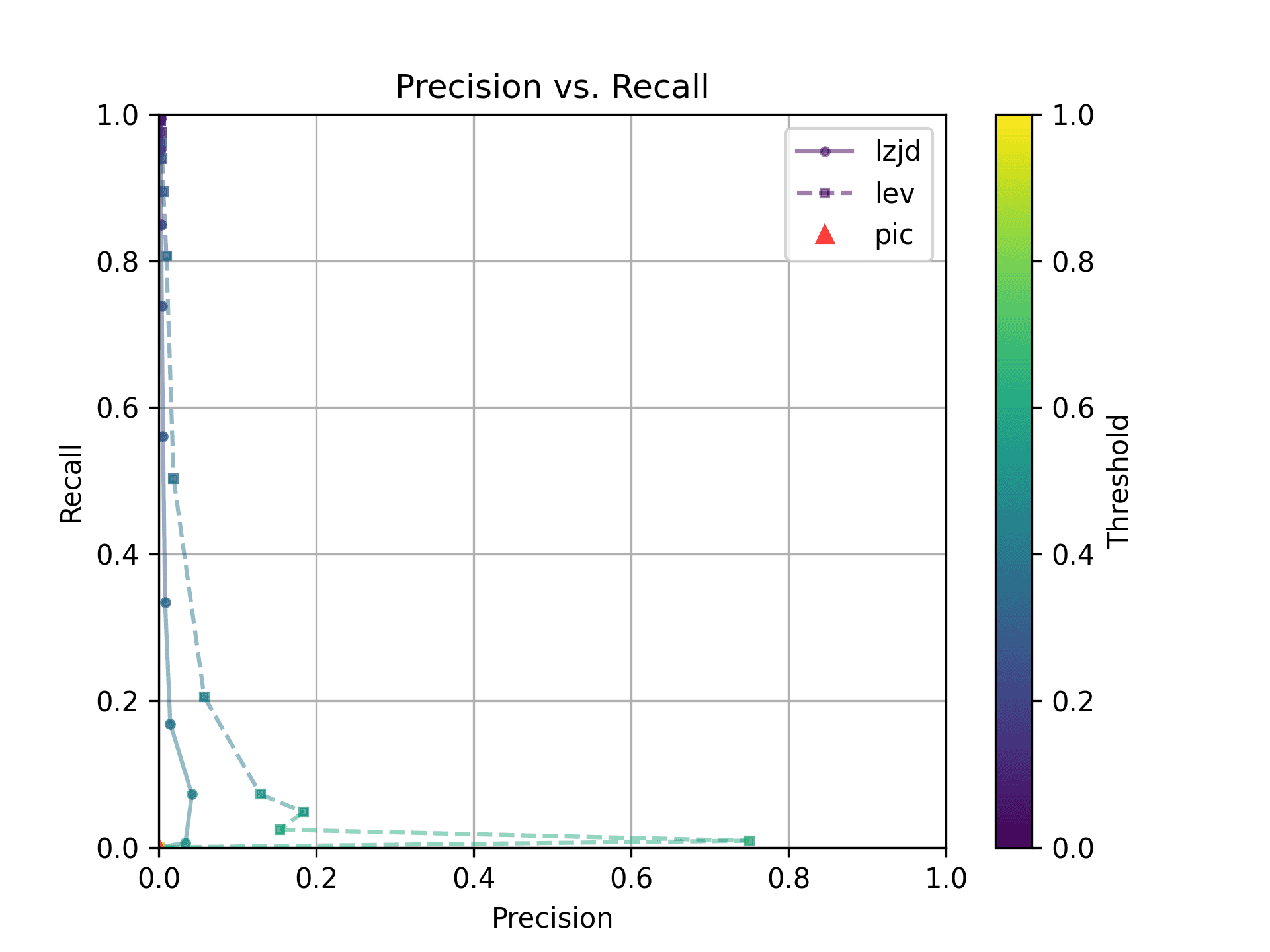
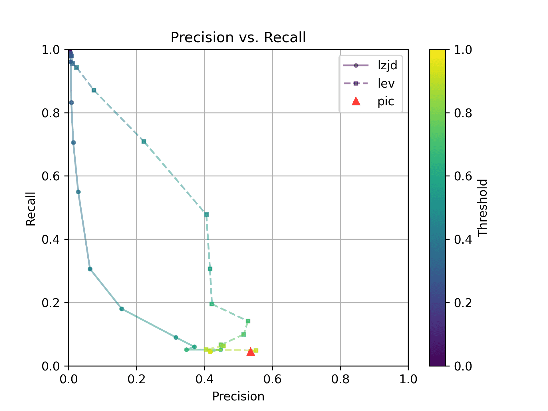
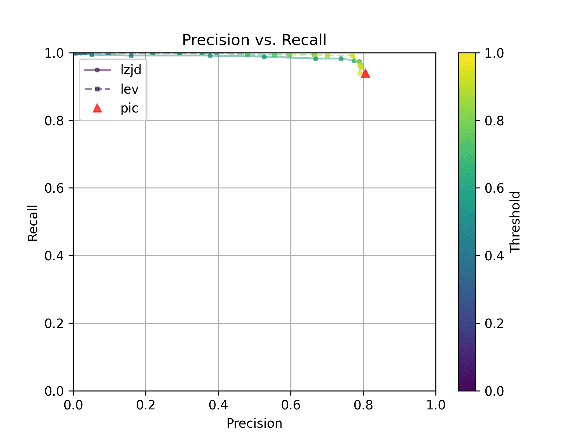
How do LZJD and LEV do? Well, that's a bit harder to quantify, because we have to pick a similarity threshold at which we consider the function to be "the same". For example, at a threshold of 0.8, we'd consider a pair of functions to be the same if they had a similarity score of 0.8 or higher. To communicate this information, we could output a confusion matrix for each possible threshold. Instead of doing this, I'll plot the results for a range of thresholds below:
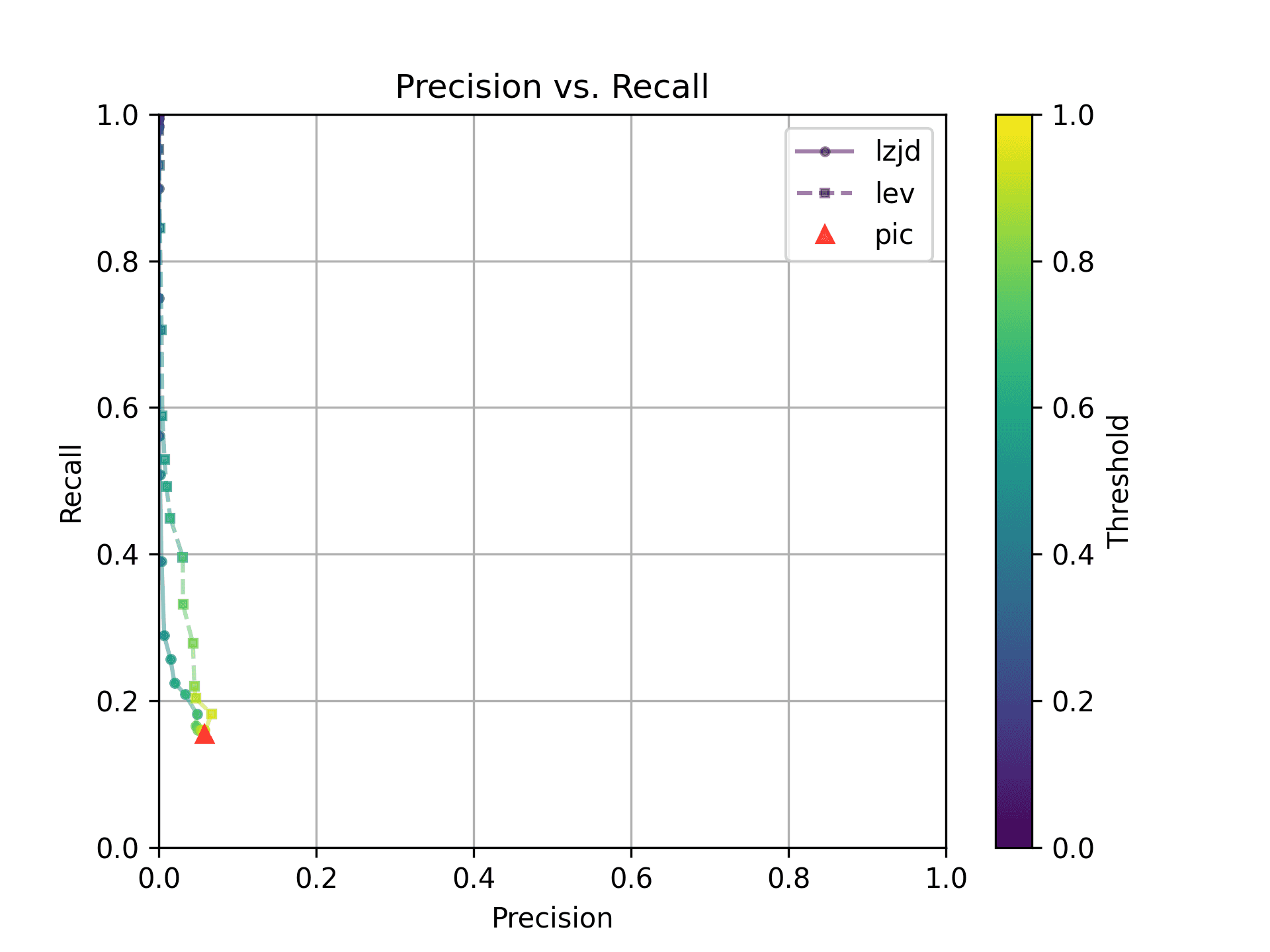
The red triangle represents the precision and recall of PIC hashing: 0.45 and 0.07 respectively, just like we got above. The solid line represents the performance of LZJD, and the dashed line represents the performance of LEV (Levenshtein distance). The color tells us what threshold is being used for LZJD and LEV. On this graph, the ideal result would be at the top right (100% recall and precision). So, for LZJD and LEV to have an advantage, it should be above or to the right of PIC hashing. But we can see that both LZJD and LEV go sharply to the left before moving up, which indicates that a substantial decrease in precision is needed to improve recall.
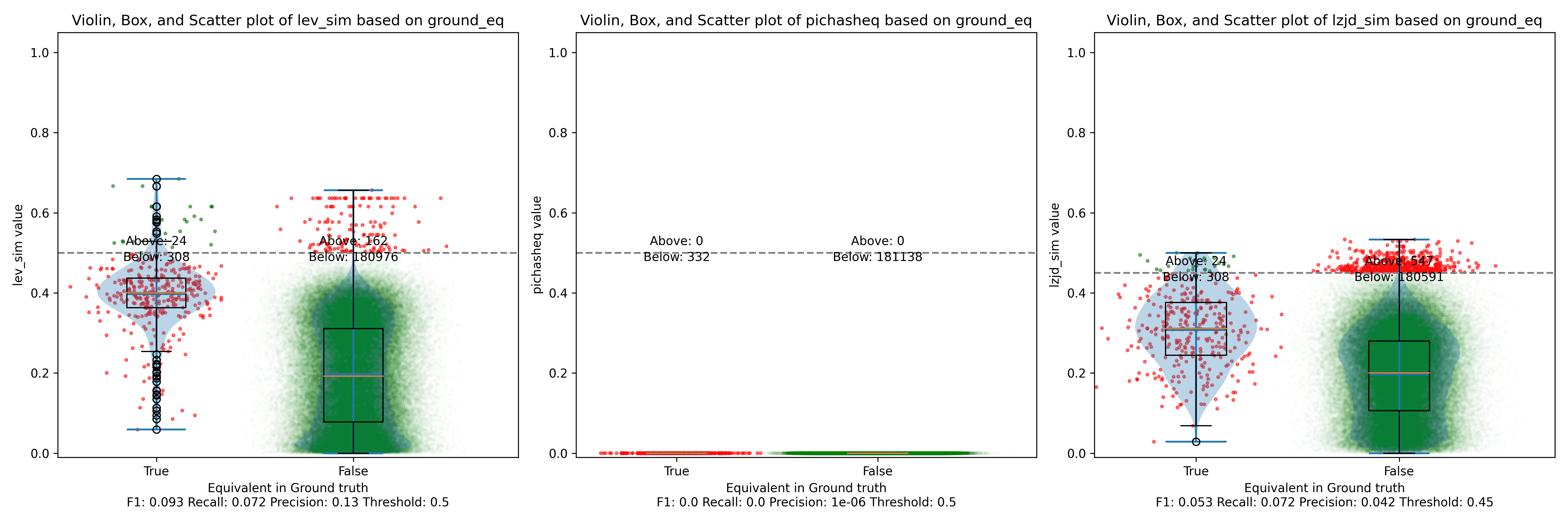
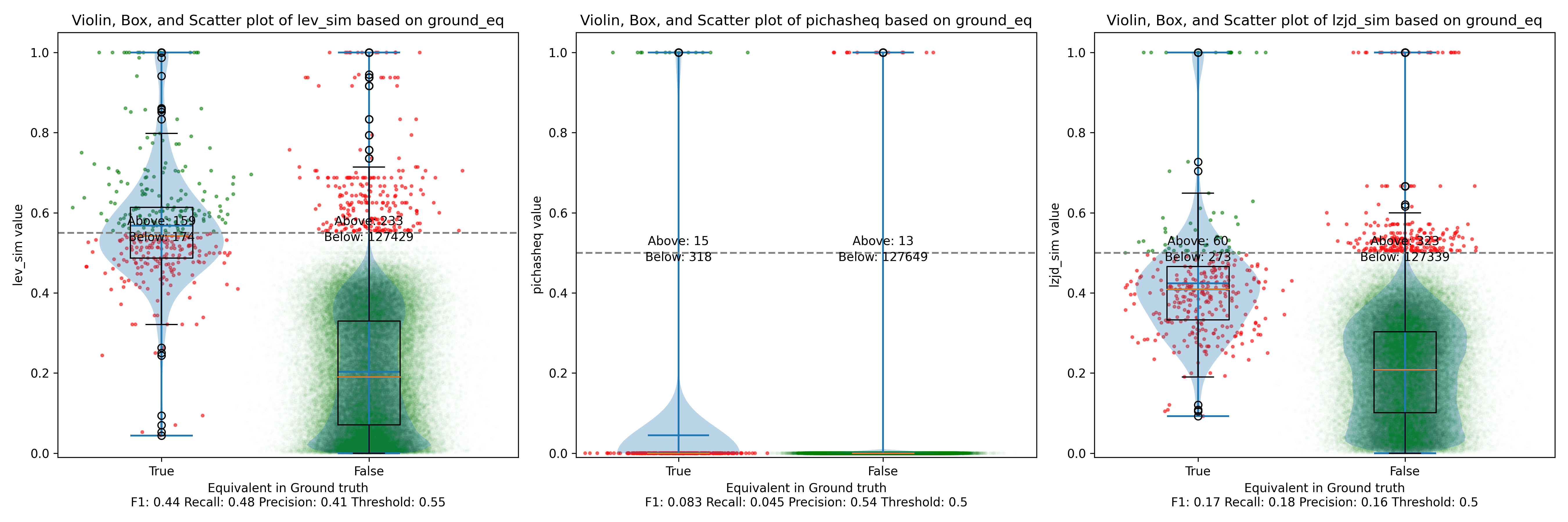
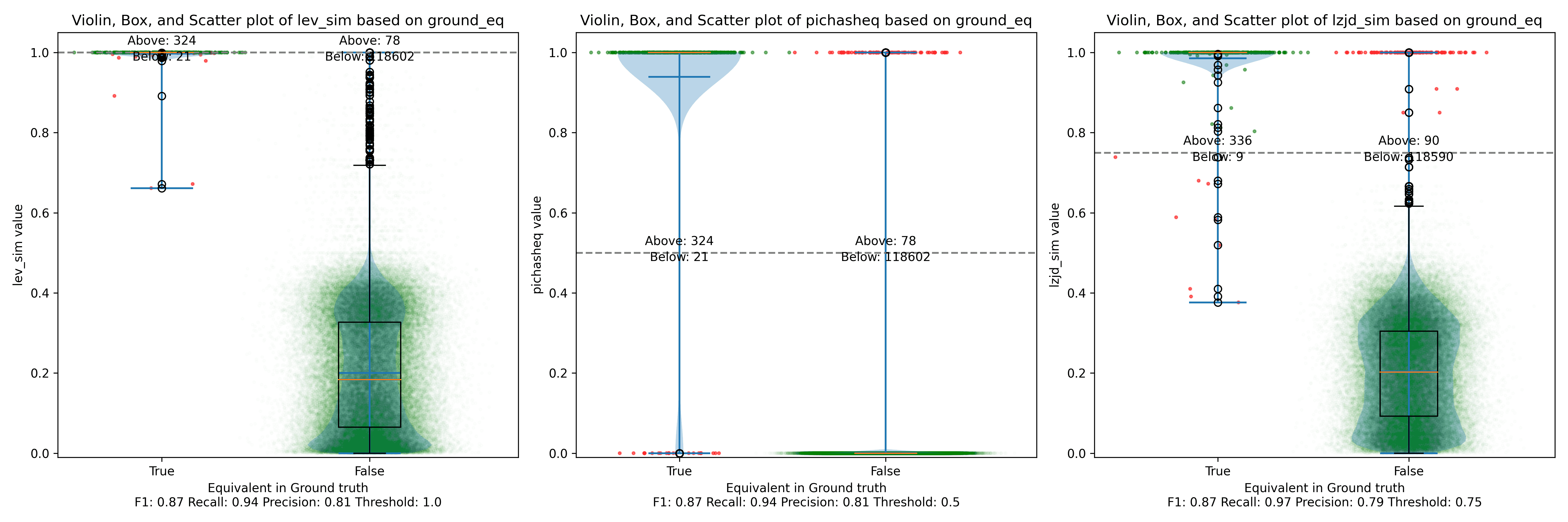
Below is what I call the violin plot. You may want to click on it to zoom in, since it's pretty wide and my blog layout is not. I also spent a long time getting that to work! There are three panels: the leftmost is for LEV, the middle is for PIC hashing, and the rightmost is for LZJD. On each panel, there is a True column, which shows the distribution of similarity scores for equivalent pairs of functions. There is also a False column, which shows the distribution scores for non-equivalent pairs of functions. Since PIC hashing does not provide a similarity score, we consider every pair to be either equivalent (1.0) or not (0.0). A horizontal dashed line is plotted to show the threshold that has the highest F1 score (i.e., a good combination of both precision and recall). Green points indicate function pairs that are correctly predicted as equivalent or not, whereas red points indicate mistakes.
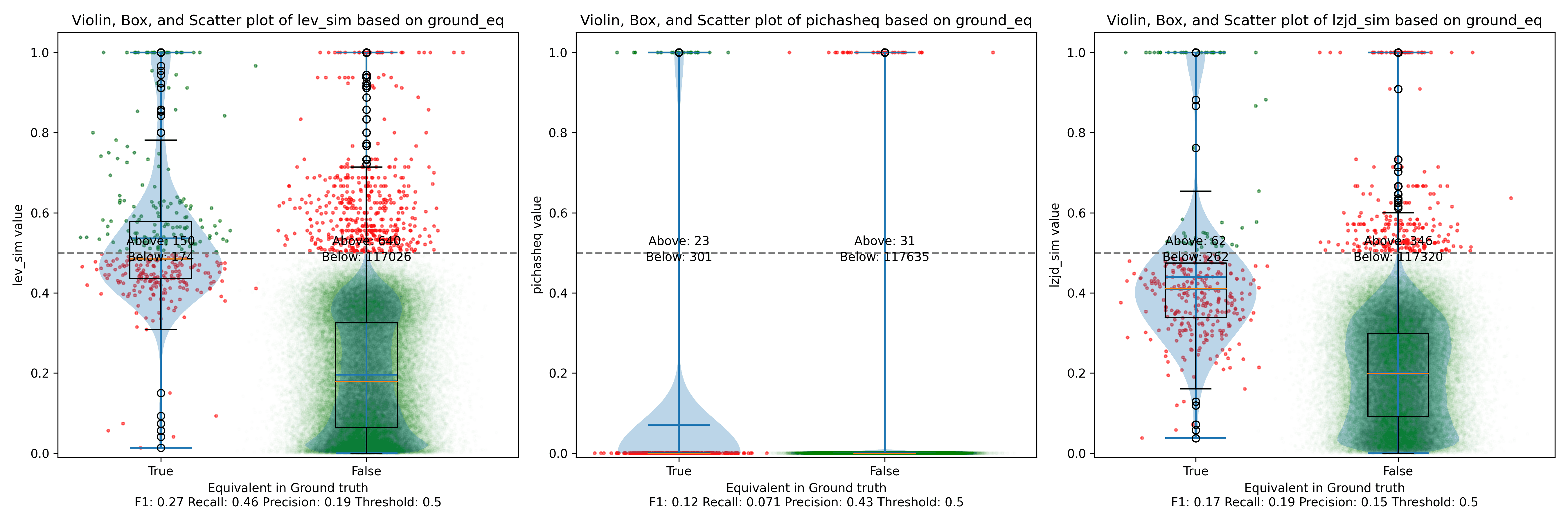
I like this visualization because it shows how well each similarity metric differentiates the similarity distributions of equivalent and non-equivalent function pairs. Obviously, the hallmark of a good similarity metric is that the distribution of equivalent functions should be higher than non-equivalent functions! Ideally, the similarity metric should produce distributions that do not overlap at all, so we could draw a line between them. In practice, the distributions usually intersect, and so instead we're forced to make a trade-off between precision and recall, as can be seen in the above Precision vs. Recall graph.
Overall, we can see from the violin plot that LEV and LZJD have a slightly
higher F1 score (reported at the bottom of the violin plot), but none of these
techniques are doing a great job. This implies that gcc and clang produce
code that is quite different syntactically.
Experiment 1b: openssl 1.1.1w Compiled With Different Optimization Levels
The next comparison I did was to compile openssl 1.1.1w with gcc -g and
optimization levels -O0, -O1, -O2, -O3.
-O0 and -O3
Let's start with one of the extremes, comparing -O0 and -O3:
The first thing you might be wondering about in this graph is Where is PIC hashing? Well, it's there at (0, 0) if you look closely. The violin plot gives us a little more information about what is going on.
Here we can see that PIC hashing made no positive predictions. In other
words, none of the PIC hashes from the -O0 binary matched any of the PIC
hashes from the -O3 binary. I included this problem because I thought it
would be very challenging for PIC hashing, and I was right! But after some
discussion with Cory, we realized something fishy was going on. To achieve a
precision of 0.0, PIC hashing can't find any functions equivalent. That
includes trivially simple functions. If your function is just a ret
there's not much optimization to do.
Eventually, I guessed that the -O0 binary did not use the
-fomit-frame-pointer option, whereas all other optimization levels do. This
matters because this option changes the prologue and epilogue of every
function, which is why PIC hashing does so poorly here.
LEV and LZJD do slightly better again, achieving low (but non-zero) F1 scores. But to be fair, none of the techniques do very well here. It's a difficult problem.
-O2 and -O3
On the much easier extreme, let's look at -O2 and -O3.

Nice! PIC hashing does pretty well here, achieving a recall of 0.79 and a precision of 0.78. LEV and LZJD do about the same. However, the Precision vs. Recall graph for LEV shows a much more appealing trade-off line. LZJD's trade-off line is not nearly as appealing, as it's more horizontal.
You can start to see more of a difference between the distributions in the violin plots here in the LEV and LZJD panels.
I'll call this one a tie.
-O1 and -O2
I would also expect -O1 and -O2 to be fairly similar, but not as similar as
-O2 and -O3. Let's see:

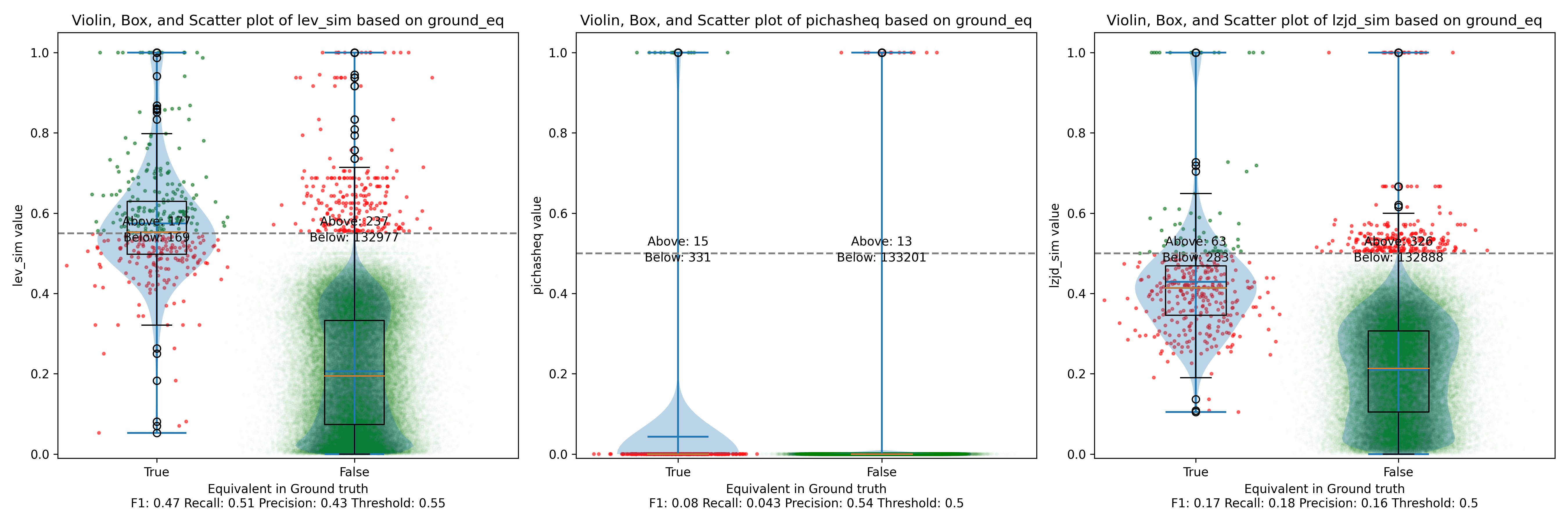
The Precision vs. Recall graph is very interesting. PIC hashing starts at a precision of 0.54 and a recall of 0.043. LEV in particular shoots straight up, indicating that by lowering the threshold, it is possible to increase recall substantially without losing much precision. A particularly attractive trade-off might be a precision of 0.43 and a recall of 0.51. This is the type of trade-off I was hoping for in fuzzy hashing.
Unfortunately, LZJD's trade-off line is again not nearly as appealing, as it curves in the wrong direction.
We'll say this is a pretty clear win for LEV.
-O1 and -O3
Finally, let's compare -O1 and -O3, which are different, but both have the
-fomit-frame-pointer option enabled by default.
These graphs look almost identical to comparing -O1 and -O2; I guess the
difference between -O2 and -O3 is really pretty minor. So it's again a win for LEV.
Experiment 2: Different openssl Versions
The final experiment I did was to compare various versions of openssl. This experiment was suggested by Cory, who thought it was reflective of typical malware RE scenarios. The idea is that the malware author released Malware 1.0, which you RE. Later, the malware changes a few things and releases Malware 1.1, and you want to detect which functions did not change so that you can avoid REing them again.
We looked at a few different versions of openssl:
| Version | Release Date | Months In Between |
|---|---|---|
| 1.0.2u | Dec 20, 2019 | N/A |
| 1.1.1 | Sep 11, 2018 | N/A |
| 1.1.1q | Oct 12, 2022 | 49 |
| 1.1.1v | Aug 1, 2023 | 9 |
| 1.1.1w | Sep 11, 2023 | 1 |
For each version, I compiled them using gcc -g -O2.
openssl 1.0 and 1.1 are different minor versions of openssl. As explained here,
Letter releases, such as 1.0.2a, exclusively contain bug and security fixes and no new features.
So, we would expect that openssl 1.0.2u is fairly different than any 1.1.1 version. And we would expect that in the same minor version, 1.1.1 would be similar to 1.1.1q, but would be more different than 1.1.1w.
Experiment 2a: openssl 1.0.2u vs 1.1.1w
As before, let's start with the most extreme comparison: 1.0.2u vs 1.1.1w.
Perhaps not too surprisingly, because the two binaries are quite different, all three techniques struggle. We'll say this is a three way tie.
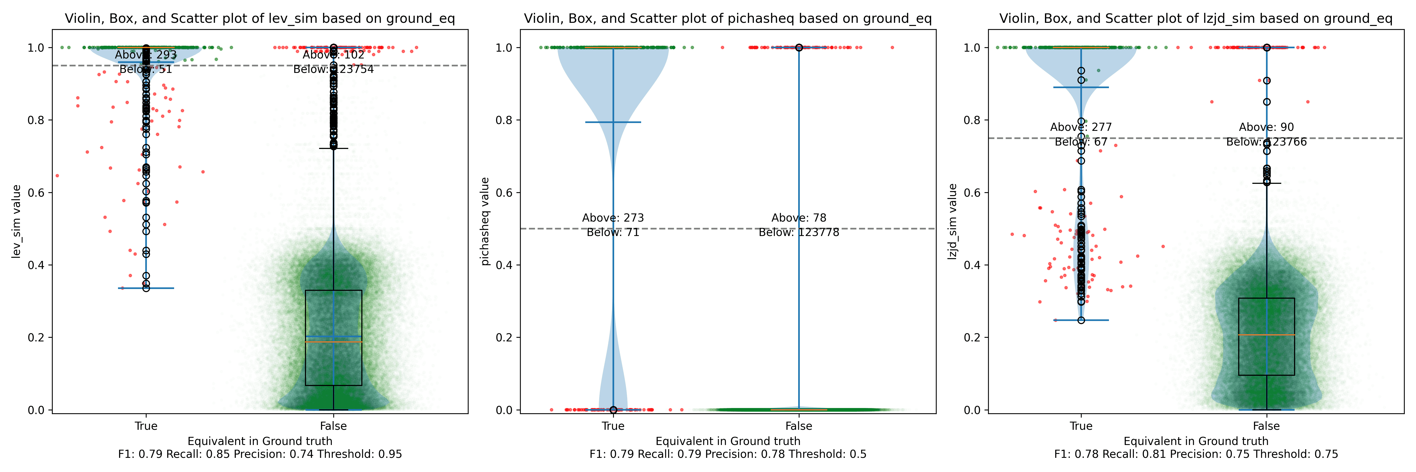
Experiment 2b: openssl 1.1.1 vs 1.1.1w
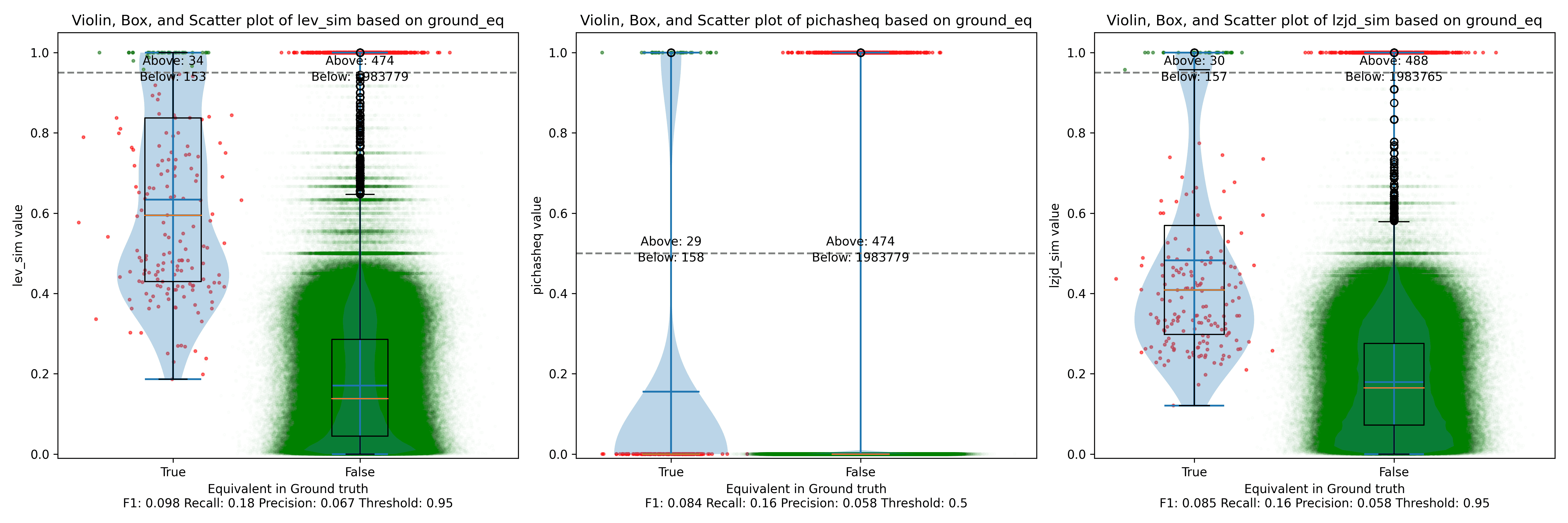
Now let's look at the original 1.1.1 release from September 2018, and compare to the 1.1.1w bugfix release from September 2023. Although a lot of time has passed between the releases, the only differences should be bug and security fixes.

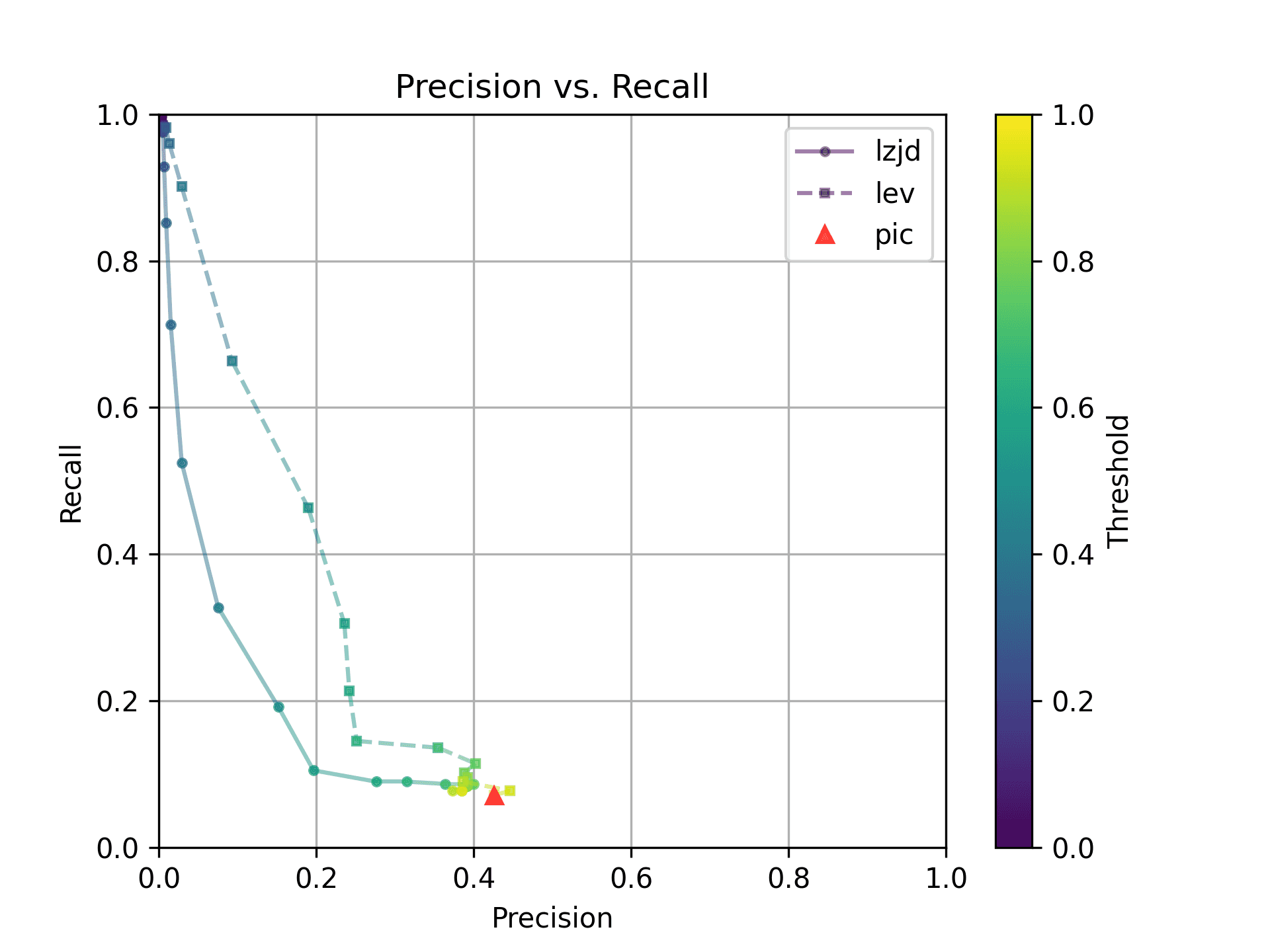
All three techniques do much better on this experiment, presumably because there are far fewer changes. PIC hashing achieves a precision of 0.75 and a recall of 0.71. LEV and LZJD go almost straight up, indicating an improvement in recall with minimal trade-off in precision. At roughly the same precision (0.75), LZJD achieves a recall of 0.82, and LEV improves it to 0.89.
LEV is the clear winner, with LZJD also showing a clear advantage over PIC.
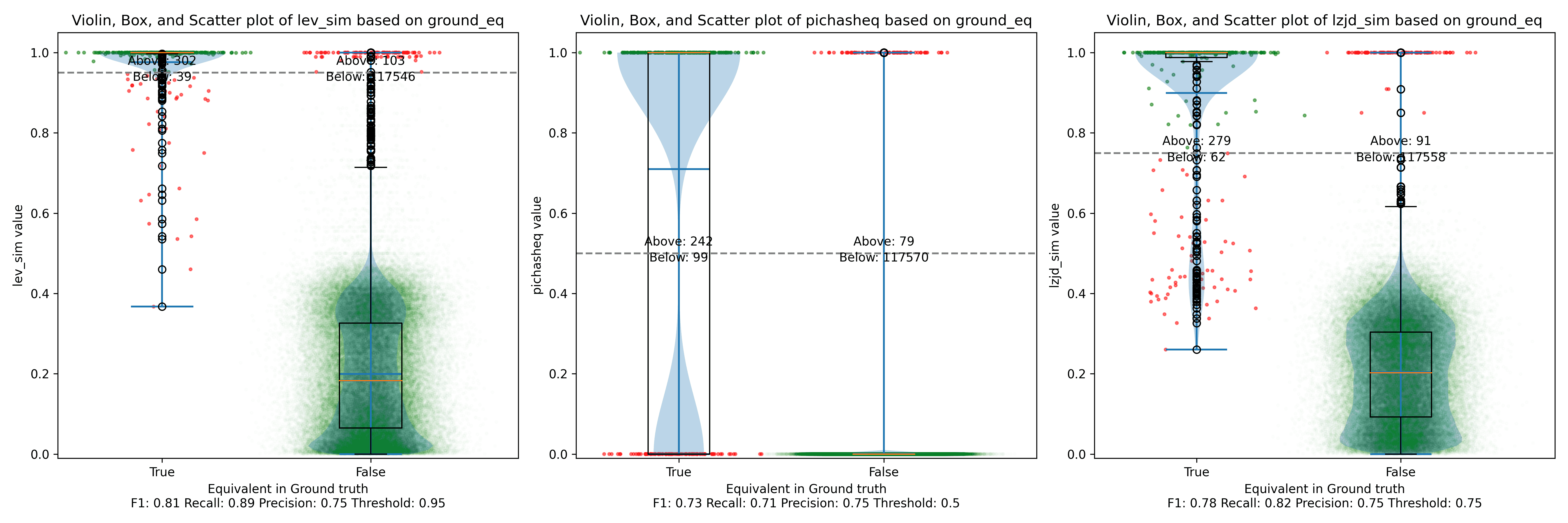
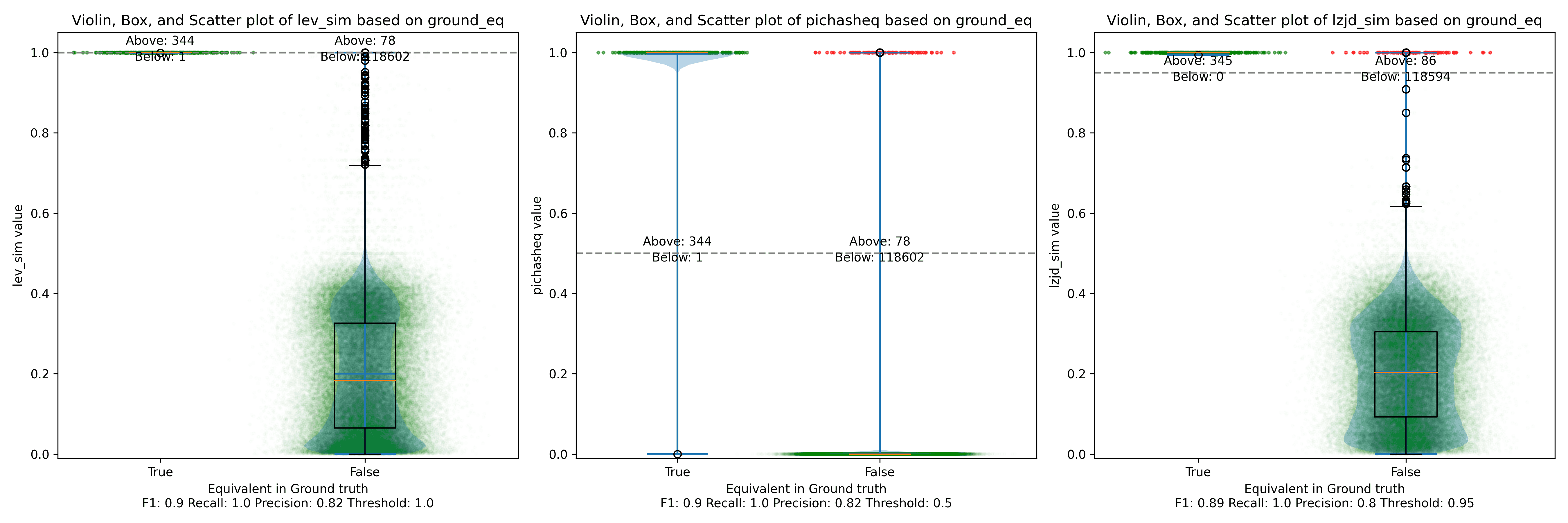
Experiment 2c: openssl 1.1.1q vs 1.1.1w
Let's continue looking at more similar releases. Now we'll compare 1.1.1q from July 2022 to 1.1.1w from September 2023.
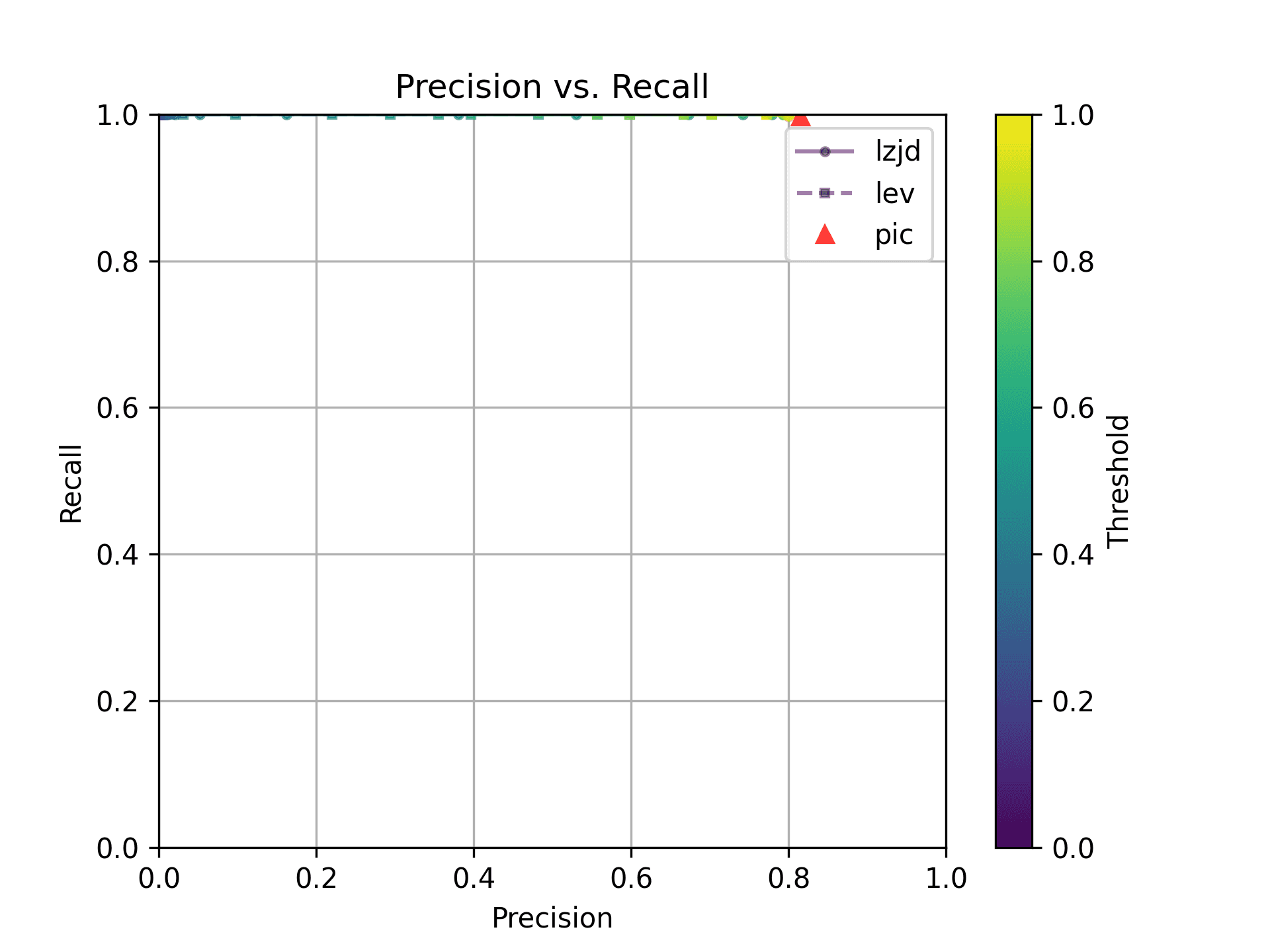
As can be seen in the Precision vs. Recall graph, PIC hashing starts at an impressive precision of 0.81 and a recall of 0.94. There simply isn't a lot of room for LZJD or LEV to make an improvement.
This is a three way tie.
Experiment 2d: openssl 1.1.1v vs 1.1.1w
Finally, we'll look at 1.1.1v and 1.1.1w, which were released only a month apart.
Unsurprisingly, PIC hashing does even better here, with a precision of 0.82 and a recall of 1.0 (after rounding)! Again, there's basically no room for LZJD or LEV to improve.
This is another three way tie.
Conclusion
Thresholds in Practice
We saw some scenarios where LEV and LZJD outperformed PIC hashing. But it's important to realize that we are conducting these experiments with ground truth, and we're using the ground truth to select the optimal threshold. You can see these thresholds listed at the bottom of each violin plot. Unfortunately, if you look carefully, you'll also notice that the optimal thresholds are not always the same. For example, the optimal threshold for LZJD in the "openssl 1.0.2u vs 1.1.1w" experiment was 0.95, but it was 0.75 in the "openssl 1.1.1q vs 1.1.1w" experiment.
In the real world, to use LZJD or LEV, you need to select a threshold. Unlike in these experiments, you could not select the optimal one, because you would have no way of knowing if your threshold was working well or not! If you choose a poor threshold, you might get substantially worse results than PIC hashing!
PIC Hashing is Pretty Good
I think we learned that PIC hashing is pretty good. It's not perfect, but it generally provides excellent precision. In theory, LZJD and LEV can perform better in terms of recall, which is nice, but in practice, it's not clear that they would because you would not know which threshold to use.
And although we didn't talk much about performance, PIC hashing is very fast. Although LZJD is much faster than LEV, it's still not nearly as fast as PIC.
Imagine you have a database of a million malware function samples, and you have a function that you want to look up in the database. For PIC hashing, this is just a standard database lookup, which can benefit from indexes and other precomputation techniques. For fuzzy hash approaches, we would need to invoke the similarity function a million times each time we wanted to do a database lookup.
There's a Limit to Syntactic Similarity
Remember that we used LEV to represent the optimal similarity based on the edit distance of instruction bytes. That LEV did not blow PIC out of the water is very telling, and suggests that there is a fundamental limit to how well syntactic similarity based on instruction bytes can perform. And surprisingly to me, PIC hashing appears to be pretty close to that limit. We saw a striking example of this limit when the frame pointer was accidentally omitted, and more generally, all syntactic techniques struggle when the differences become too great.
I wonder if any variants, like computing similarities over assembly code instead of executable code bytes, would perform any better.
Where Do We Go From Here?
There are of course other strategies for comparing similarity, such as incorporating semantic information. Many researchers have studied this. The general downside to semantic techniques is that they are substantially more expensive than syntactic techniques. But if you're willing to pay the price, you can get better results. Maybe in a future blog post we'll try one of these techniques out, such as the one my contemporary and friend Wesley Jin proposed in his dissertation.
While I was writing this blog post, Ghidra 11.0 also introduced BSim:
A major new feature called BSim has been added. BSim can find structurally similar functions in (potentially large) collections of binaries or object files. BSim is based on Ghidra's decompiler and can find matches across compilers used, architectures, and/or small changes to source code.
Another interesting question is whether we can use neural learning to help compute similarity. For example, we might be able to train a model to understand that omitting the frame pointer does not change the meaning of a function, and so shouldn't be counted as a difference.
I've been feeling left behind by all the exciting news surrounding AI, so I've been quietly working on a project to get myself up to speed with some modern Transformers models for NLP. This project is mostly a learning exercise, but I'm sharing it in the hopes that it is still interesting!
Background: Functions, Methods and OOAnalyzer
One of my favorite projects is OOAnalyzer, which is part of SEI's Pharos static binary analysis framework. As the name suggests, it is a binary analysis tool for analyzing object-oriented (OO) executables to learn information about their high level structure. This structure includes classes, the methods assigned to each class, and the relationships between classes (such as inheritance). What's really cool about OOAnalyzer is that it is built on rules written in Prolog -- yes, Prolog! So it's both interesting academically and practically; people do use OOAnalyzer in practice. For more information, check out the original paper or a video of my talk.
Along the way to understanding a program's class hierarchy, OOAnalyzer needs to solve many smaller problems. One of these problems is: Given a function in an executable, does this function correspond to an object-oriented method in the source code? In my humble opinion, OOAnalyzer is pretty awesome, but one of the yucky things about it is that it contains many hard-coded assumptions that are only valid for Microsoft Visual C++ on 32-bit x86 (or just x86 MSVC to save some space!)
It just so happens that on
this compiler and platform, most OO methods use the thiscall calling
convention, which passes a pointer to the this object in the ecx register. Below is an interactive Godbolt example that shows a simple method mymethod being compiled by x86 MSVC. You can see on line 7 that the thisptr is copied from ecx onto the stack at offset -4. On line 9, you can see that arg is passed on the stack. In contrast, on line 20, myfunc only receives its argument on the stack, and does not access ecx.
(Note that this assembly code comes from the compiler and includes the name of functions, which makes it obvious whether a function corresponds to an OO method. Unfortunately this is not the case when reverse engineering without access to source code!)
Because most non-thisptr arguments are passed on the stack in x86 MSVC, but the thisptr is passed in ecx, seeing an argument in the ecx register is highly suggestive (but not definitive) that the function corresponds to an OO
method. OOAnalyzer has a variety of heuristics based on this notion that tries
to determine whether a function corresponds to an OO method. These work well,
but they're specific to x86 MSVC. What if we wanted to
generalize to other compilers? Maybe we could learn to do that. But first,
let's see if we can learn to do this for x86 MSVC.
Learning to the Rescue
Let's play with some machine learning!
Step 1: Create a Dataset
You can't learn without data, so the first thing I had to do was create a dataset. Fortunately, I already had a lot of useful tools and projects for generating ground truth about OO programs that I could reuse.
BuildExes
The first project I used was BuildExes. This is a project that takes several test programs that are distributed as part of OOAnalyzer and builds them with many versions of MSVC and a variety of compiler options. The cute thing about BuildExes is that it uses Azure pipelines to install different versions of MSVC using the Chocolatey package manager and perform the compilations. Otherwise we'd have to install eight MSVC versions, which sounds like a pain to me. BuildExes uses a mix of publicly available Chocolatey packages and some that I created for older versions of MSVC that no one else cares about 🤣.
When BuildExes runs on Azure pipelines, it produces an artifact consisting of a large number of executables that I can use as my dataset.
Ground Truth
As part of our evaluations for the OOAnalyzer paper, we wrote a variety of scripts that extracted ground truth information out of PDB debugging symbols files (which, conveniently, are also included in the BuildExes artifact!) These scripts aren't publicly available, but they aren't top secret and we've shared them with other researchers. They essentially call a tool to decode PDB files into a textual representation and then parse the results.
Putting it Together
Here is the script that produces the ground truth
dataset.
It's a bit obscure, but it's not very complicated. Basically, for each executable in the BuildExes
project, it reads the ground truth file, and also uses the bat-dis
tool from the ROSE Binary
Analysis Framework to
disassemble the program.
The initial dataset is available on 🤗 HuggingFace. Aside: I love that 🤗 HuggingFace lets you browse datasets to see what they look like.
Step 2: Split the Data
The next step is to split the data into training and test sets. In ML, the best practice is generally to ensure that there is no overlap between the training and test sets. This is so that the performance of a model on the test set represents performance on "unseen examples" that the model has not been trained on. But this is tricky for a few reasons.
First, software is natural, which means that we can expect that distinct programmers will naturally write the same code over and over again. If a function is independently written multiple times, should it really count as an "previously seen example"? Unfortunately, we can't distinguish when a function is independently written multiple times or simply copied. So when we encounter a duplicate function, what should we do? Discard it entirely? Allow it to be in both the training and test sets? There is a related question for functions that are very similar. If two functions only differ by an identifier name, would knowledge of one constitute knowledge of the other?
Second, compilers introduce a lot of functions that are not written by the programmer, and thus are very, very common. If you look closely at our dataset, it is actually dominated by compiler utility functions and functions from the standard library. In a real-world setting, it is probably reasonable to assume that an analyst has seen these before. Should we discard these, or allow them to be in both the training and test sets, with the understanding that they are special in some way?
Constructing a training and test split has to take into account these questions. I actually created an additional dataset that splits the data via different mechanisms.
I think the most intuitively correct one is what I call splitting by library
functions. The idea is quite simple. If a function name appears in the
compilation of more than one test program, we call it a library function. For
example, if we compile oo2.cpp and oo3.cpp to oo2.exe and oo3.exe
respectively, and both executables contain a function called
msvc_library_function, then that function is probably introduced by the
compiler or standard library, and we call it a library function. If function
oo2_special_fun only appears in oo2.exe and no other executables, then we
call it a non-library function. We then split the data into training and test
sets such that the training set consists only of library functions, and the test
set consists only of non-library functions. In essence, we train on the commonly
available functions, and test on the rare ones.
This idea isn't perfect, but it works pretty well, and it's easy to understand and justify. You can view this split here.
Step 3: Fine-tune a Model
Now that we have a dataset, we can fine-tune a model. I used the huggingface/CodeBERTa-small-v1 model on 🤗 HuggingFace as a base model. This is a model that was trained on a large corpus of code, but that is not trained on assembly code (and we will see some evidence of this).
My model, which I fine-tuned with the training split using the "by library" method described above, is available as ejschwartz/oo-method-test-model-bylibrary. It attains 94% accuracy on the test set, which I thought was pretty good. I suspect that OOAnalyzer performs similarly well.
If you are familiar with the 🤗 Transformers library, it's actually quite easy to use my model (or someone else's). You can actually click on the "Use in Transformers" button on the model page, and it will show you the Python code to use. But if you're a mere mortal, never fear, as I've created a Space for you to play with, which is embedded here:
If you want, you can upload your own x86 MSVC executable. But if you don't
have one of those lying around, you can just click on one of the built-in example
executables at the bottom of the space (ooex8.exe and
ooex9.exe). From there, you can select a function from the dropdown menu to
see its disassembly, and the model's opinion of whether it is a class method or
not. If the assembly code is too long for the model to process, you'll currently encounter an error.
Here's a recording of what it looks like:
If you are very patient, you can also click on "Interpret" to run Shapley interpretation, which will show which tokens are contributing the most. But it is slow. Very slow. Like five minutes slow. It also won't give you any feedback or progress (sigh -- blame gradio, not me).
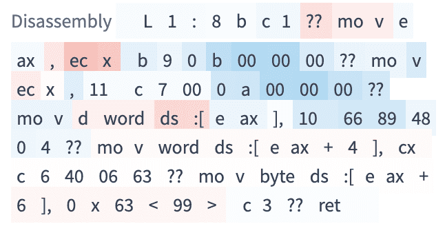
Here's an example of an interpretation. The dark red tokens contribute more to
method-ness and dark blue tokens contribute to function-ness. You can also see that
registers names are not tokens in the original CodeBERT model. For instance, ecx
and is split into ec and x, which the model learns to treat as a pair. It's
not a coincidence that the model learned that ecx is indicative of a method,
as this is a rule used in OOAnalyzer as well. It's also somewhat interesting that the model views sequences of zero bytes in the binary code as being indicative of function-ness.
Looking Forward
Now that we've shown we can relearn a heuristic that is already included in OOAnalyzer, this raises a few other questions:
-
One of the "false positives" of the
ecxheuristics is thefastcallcalling convention, which also uses theecxregister. We should ensure that the dataset contains functions with this calling convention (and others), since they do occur in practice. -
What other parts of OOAnalyzer can we learn from examples? How does the accuracy of learned properties compare to the current implementation?
-
Can we learn to distinguish functions and methods for other architectures and compilers? Unfortunately, one bottleneck here is that our ground truth scripts only work for MSVC. But this certainly isn't an insurmountable problem.
I'm happy to announce that a paper written with my colleagues, A Generic Technique for Automatically Finding Defense-Aware Code Reuse Attacks, will be published at ACM CCS 2020. This paper is based on some ideas I had while I was finishing my degree that I did not have time to finish. Fortunately, I was able to find time to work on it again at SEI, and this paper is the result. A pre-publication copy is available from the publications page.
One of the aspects I like about my job as a researcher at SEI is that I split my time between being an academic researcher and a software engineer. For example, a few years ago, my colleagues and I published a paper on how to employ logic programming to recover object-oriented abstractions from an executable. I was very proud of that paper (and still am!) because it introduces some interesting new approaches to performing binary analysis, and yet is also a usable tool (OOAnalyzer) that people are actually using to reverse engineer real software.
Although basing our system on logic programming made for an interesting paper, it also made it challenging to scale OOAnalyzer to very large and complex executables. We strugged from the beginning to achieve reasonable performance, and eventually concluded that we had to aggressively use tabling in order to achieve reasonable performance. At a high level, tabling is memoization for Prolog. Prolog does have side-effects, though, and part of the challenge for tabling implementations is to make sure that the tables are consistent.
One of the leading Prolog implementations with tabling support is XSB Prolog, which OOAnalyzer has been using since the beginning. Teri Swift, one of the XSB developers, and the leading expert on Prolog tabling, really helped us get enough performance to be able to write our paper. We were able to analyze some large and interesting programs, including mysql.exe, the MySQL client program. The largest program we were able to test in our paper was over 5 MiB.
Unfortunately, there were many programs that we weren't able to test successfully as well. One of these that really stuck in my mind was mysqld.exe. In our paper, we were able to run successfully on mysql.exe, the MySQL client program, but mysqld.exe, the daemon was much larger (22 MiB vs 5 MiB), and remained elusive.
A while after we published our paper, we started working again with Teri Swift, who was helping Jan Wielemaker of SWI Prolog add support for tabling to SWI Prolog. Teri and Jan wanted to use OOAnalyzer as a test case to make sure that SWI Prolog's tabling implementation was working correctly. Since this would mean that OOAnalyzer would have another supported Prolog engine, this was a win-win situation for us! Jan graciously helped us get OOAnalyzer running on SWI, which was useful in its own right. He also developed some invaluable debugging tools to help us understand what tabling is doing behind the scenes.
These tools, combined with a lot of profiling and rewriting iterations, eventually allowed us to improve performance bottlenecks to the point that we could successfully reason through mysqld.exe and other similarly large programs! Along the way, we battled performance bottlenecks, memory that would not be reclaimed, and other problems. But now we can analyze mysqld.exe in about 18 hours, and only using about 12 GiB of memory. And what is encouraging is that even near the end of reasoning about such a large program, the tool is still making new inferences fairly quickly.
These updates are available in the latest release of the Pharos repository. My colleague Cory Cohen recently wrote a tutorial on how to run OOAnalyzer on large executables, with all of the tricks we have learned over the years.
While working with Teri and Jan, I very slowly began to understand some of the underlying problems that would cause performance to degrade in large programs. One of the problems was that, to maintain consistency, the tabling implementation would re-compute tables from scratch. For most tables, this could be done quickly. But for others, it would take up huge amounts of time. I also realized that because of the structure of our problem, which incrementally learns new conclusions over time, the recomputations were not really needed.
I created a work-around in Prolog that I call "trigger rules". I rewrote the most expensive OOAnalyzer rules to be triggered when dependent facts were introduced, which avoided the costly (and unnecessary) recomputation of the table for all values. The conversion process is fragile and manual, but it proved that if we could avoid the costly recomputations, OOAnalyzer's performance would scale pretty well.
More recently, we've been working with Jan on some a tabling method that avoids the costly recomputations (and also avoids the fragile, error-prone manual transformations that I needed to make for trigger rules). The new type of tabling is called monotonic tabling. There are still some kinks to work out, but we are optimistic that this will further improve the performance of OOAnalyzer and make it easier to maintain.
And of course, monotonic tabling will probably make for an interesting subject of a new paper. So we've now come full circle. We wrote the research paper on OOAnalyzer. This led us to engineering challenges. And to solve the engineering challenges, it brought us back to a new research problem.
My colleagues and I wrote a survey paper on fuzzing entitled The Art, Science, and Engineering of Fuzzing: A Survey. Late last year this was accepted to appear in the IEEE Transactions on Software Engineering journal, but has not been officially published to date. We also recently learned that it will appear at ICSE 2020. As usual, you can download it from the publications page.
My colleagues and I finished the camera ready version of our DIRE paper on variable name recovery. Although there's no code released at this time, I'm hoping to release a proof of concept Hex-Rays plugin.
Powered with by Gatsby 5.0